New in SG-Lib 3.8
VLdistance(VL)- returns a distance list - but is different from VLnorm |
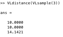 |
% VLdistance(VL) - returns a distance list - but is different from VLnorm % (by Tim Lueth, VLFL-Lib, 2017-MAI-24 as class: ANALYTICAL GEOMETRY) % % Version 4.0 is 10-20 times faster than 3.9 % VLnorm - vertex normal vector; not defined for the first value % VLdistance - vertex distance vector; not defined for the last value % The results seem to be circulated by one % VLdistance is looking forward % VLnorm is looking backward (Status of: 2017-07-09) % % Introduced first in SolidGeometry 3.8 % % See also: NLnorm, VLangle % % [DL,DVL]=VLdistance(VL) % === INPUT PARAMETERS === % VL: Vertex list % === OUTPUT RESULTS ====== % DL: Distance list % DVL: Distance vector list % % EXAMPLE: % VLnorm(VLsample(3)) % VLdistance(VLsample(3)) % % See also: NLnorm, VLangle % |
PLof3dist(d1,d2,d3,srt)- creates a 3P Tracker geometry using the given distances |
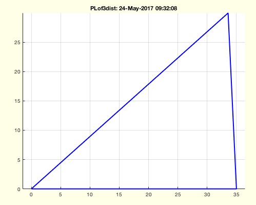 |
% PLof3dist(d1,d2,d3,srt) - creates a 3P Tracker geometry using the given distances % (by Tim Lueth, VLFL-Lib, 2017-MAI-24 as class: ANALYTICAL GEOMETRY) % % See also: cross2circ % % [PL,n,d3]=PLof3dist(d1,d2,[d3,srt]) % === INPUT PARAMETERS === % d1: distance in x % d2: radius at second point % d3: radius at third/first point point; % srt: sort by length; default is false % === OUTPUT RESULTS ====== % PL: Point list % n: area of triangle % d3: d3 % % EXAMPLE: % PLof3dist(35,30,45) % PLof3dist(35,30,45,true) % |
SGspherelink(Lz,R1,R2,olap)- returns a spherical link |
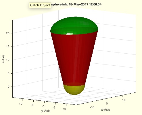 |
% SGspherelink(Lz,R1,R2,olap) - returns a spherical link % (by Tim Lueth, VLFL-Lib, 2017-MAI-18 as class: SURFACES) % % This fnctn is helpful to design more natural shaped links (Status of: % 2017-05-18) % % See also: SGsphere % % SGC=SGspherelink(Lz,[R1,R2,olap]) % === INPUT PARAMETERS === % Lz: Length in Z % R1: Upper radial values [Rx Ry Rz]; default is L/4 % R2: lower radial values [Rx Ry Rz]; default is R1 % olap: overlap of the three solids; default is 1e-3; % === OUTPUT RESULTS ====== % SGC: Final solid % % EXAMPLE: % SGspherelink(20,[5 5 5]); % Pill shape % SGspherelink(20,[5 5 0]); % Cylinder shape % SGspherelink(20,[5 2 0]); % Rod % SGspherelink(20,[5 5 10],[5 5 0]); % Jules Verne Moon Rocket Shape % SGspherelink(450,[400 200 80],[300 150 0]); % Torso shape % |
CVLofSGslices(SG,n)- returns slices as CVL (CPL including z) of a SG |
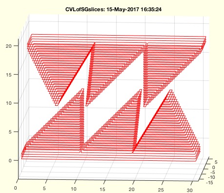 |
% CVLofSGslices(SG,n) - returns slices as CVL (CPL including z) of a SG % (by Tim Lueth, VLFL-Lib, 2017-MAI-15 as class: SLICES) % % This fnctn is useful for creating 3D printing strategies over several % slices. It also helps to reconstruct solids (Status of: 2017-05-26) % % Introduced first in SolidGeometry 3.8 % % See also: CPLofSGslice3, SGofCVLslices, CVLseparate % % CVL=CVLofSGslices(SG,[n]) % === INPUT PARAMETERS === % SG: Solid Geometry % n: number of slices; default is 10 % === OUTPUT RESULTS ====== % CVL: CPL of the slices including the relevant c coordinate % % EXAMPLE: % CVLofSGslices(SGsample(23),50) % % See also: CPLofSGslice3, SGofCVLslices, CVLseparate % |
SGunitecells(SGc)- converts all cells into one solid geometry |
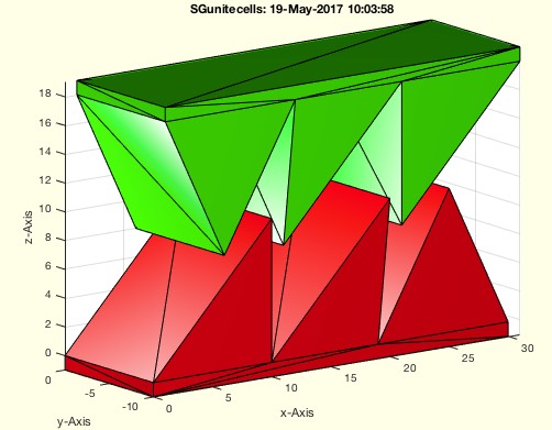 |
% SGunitecells(SGc) - converts all cells into one solid geometry % (by Tim Lueth, VLFL-Lib, 2017-MAI-15 as class: SURFACES) % % Quick and Dirty - Does not support frames yet % (Status of: 2017-05-19) % % See also: SGcat, SGcat2, VLFLofSG, SGofVLFL % % SG=SGunitecells(SGc) % === INPUT PARAMETERS === % SGc: {SGA; SGB; SGC;} % === OUTPUT RESULTS ====== % SG: SG.VL, SG.FL % % EXAMPLE: % SGunitecells(SGsample(22)) % SGunitecells(SGsample(23)) % |
PLofimcontourc(I,cent,pixs)- returns the centers of pixel coordinates in an image |
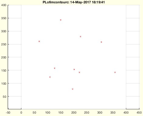 |
% PLofimcontourc(I,cent,pixs) - returns the centers of pixel coordinates in an image % (by Tim Lueth, VLFL-Lib, 2017-MAI-14 as class: CLOSED POLYGON LISTS) % % See also: CPLcontourc % % PL=PLofimcontourc(I,[cent,pixs]) % === INPUT PARAMETERS === % I: Image % cent: true= image origin is in center; default is false % pixs: size of a pixel; default is [1 1] % === OUTPUT RESULTS ====== % PL: Coordinate list of contour centers % % EXAMPLE: % I=imageofVLprojection(VL,[100 100],[0 -100 0],[0 100 0],4); % PLofimcontourc(I,true,1/4) % |
centerCPL(CPL)- returns the center of all contours of a CPL |
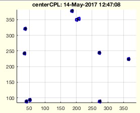 |
% centerCPL(CPL) - returns the center of all contours of a CPL % (by Tim Lueth, VLFL-Lib, 2017-MAI-14 as class: CLOSED POLYGON LISTS) % % This fnctn helps to find fiducial marker center in xray images (Status % of: 2017-05-14) % % Introduced first in SolidGeometry 3.8 % % See also: centerPL, CPLcontourc % % PL=centerCPL(CPL) % === INPUT PARAMETERS === % CPL: Closed Polygon list with several PL's % === OUTPUT RESULTS ====== % PL: List of center of CPL using centerPL % % EXAMPLE: % VL=50*rand(10,3)-25; % I=imageofVLprojection(VL,[100 100],[0 -100 0],[0 100 0],4); % CPL=CPLcontourc(double(I),1); % centerCPL(CPL) % % See also: centerPL, CPLcontourc % |
VLofimsegthres(I)- returns a VL of segmented points within an image |
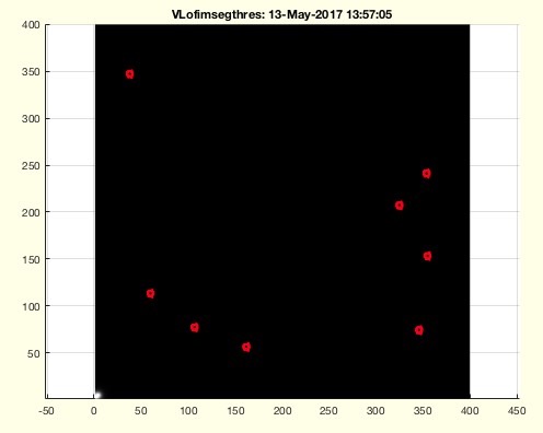 |
% VLofimsegthres(I) - returns a VL of segmented points within an image % (by Tim Lueth, VLFL-Lib, 2017-MAI-12 as class: ANALYTICAL GEOMETRY) % % This fnctn helps to find the center of features islands within an image % (Status of: 2017-05-14) % % Introduced first in SolidGeometry 3.8 % % [VLC,VLs,VL,S]=VLofimsegthres(I) % === INPUT PARAMETERS === % I: Logical Image % === OUTPUT RESULTS ====== % VLC: Vertex List of centers % VLs: size of features % VL: All feature poits % S: index list for features % % EXAMPLE: % VL=50*rand(10,3)-25; % I=imageofVLprojection(VL,[100 100],[0 -100 0],[0 100 0],4); % VLofimsegthres(I<200); % |
Tofcam(pc,pt,cup)- returns HT matrix of camera and target for a given camera point, target point, and camera up vector |
 |
% Tofcam(pc,pt,cup) - returns HT matrix of camera and target for a given camera point, target point, and camera up vector % (by Tim Lueth, VLFL-Lib, 2017-MAI-11 as class: USER INTERFACE) % % Introduced first in SolidGeometry 3.8 % % See also: Tofgca % % [T,Tt,va,ax]=Tofcam(pc,pt,cup) % === INPUT PARAMETERS === % pc: point of camera; default is campos % pt: point of target; default is camtarget % cup: cup direction ; rough; default is camup % === OUTPUT RESULTS ====== % T: Transformation of camera % Tt: Transformation of target % va: current camera angle % ax: current axis values % % EXAMPLE: % SGfigure; SGplot(SGsample(1)); pause; Tofcam % % See also: Tofgca % |
imageofVLprojection(VL,isize,pc,pt,pixnum,cup)- returns an image of a VL projection using the matlab camera view concept |
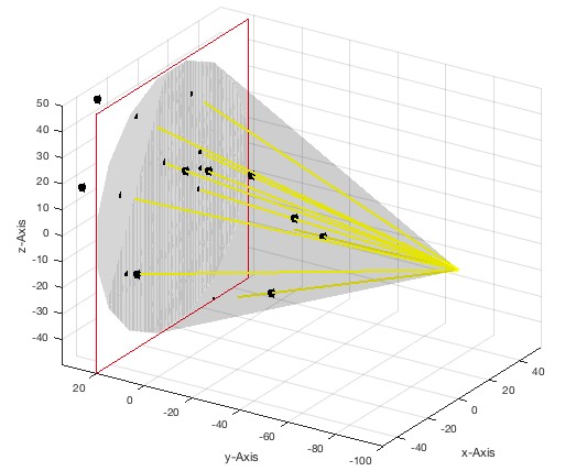 |
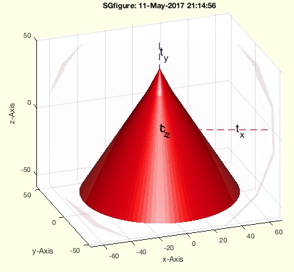
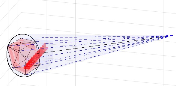
% imageofVLprojection(VL,isize,pc,pt,pixnum,cup) - returns an image of a VL projection using the matlab camera view concept % (by Tim Lueth, VLFL-Lib, 2017-MAI-11 as class: ANALYTICAL GEOMETRY) % % To get a real projection image using the graphics camera parameter it % is absolutely necessary to switch to perspective mode first (this is % part of this fnctn) before taking a snapshot (getframe); % >> set(gca,'Projection','perspective'); % The image size in mm defines the opening angle: 2*tan(alpha)=x/2 / % norm(pc-pt) % The angle alpha is the complete opening angle, same for both dimensions. % Therefor the target screen height is x = 2 * tan (alpha/2) * % norm(pc-pt) (Status of: 2017-05-12) % % Introduced first in SolidGeometry 3.8 % % See also: imwarpT % % [I,Ic,pixs,Tc,Tt,C]=imageofVLprojection([VL,isize,pc,pt,pixnum,cup]) % === INPUT PARAMETERS === % VL: Vertex list; default is a square for testing % isize: image size [x y] centered; this defines the view angle % pc: position of camera; default is [0 +100 0]; % pt: position of screen; default is [0 -100 0]; % pixnum: pixels of image; default is isize; % cup: cup vector; default is [1 0 0] % === OUTPUT RESULTS ====== % I: Grey scale matrix [0..1] % Ic: Color Matrix struct I.cdata % pixs: pixel size in mm; scaling % Tc: HT matrix of camera position % Tt: HT matrix of target position % C: SG of the perspective cone in space % % EXAMPLE: % imageofVLprojection('',[200 200],[0 -400 0],[0 100 0],1); % Original % imageofVLprojection('',[200 200],[0 -400 0],[0 100 0],2); % Dots smaller % imageofVLprojection('',[200 200],[0 -400 0],[0 200 0],2); % Dots outward % imageofVLprojection('',[200 200],[0 -400 0],[0 600 0],2); % Dots out % imageofVLprojection(100*rand(10,3)-50,[200 200],[0 -400 0],[0 600 0]); % % See also: imwarpT % |
imwarpT(I,T,scal,cent,fc)- warps an image related to a give transformation matrix |
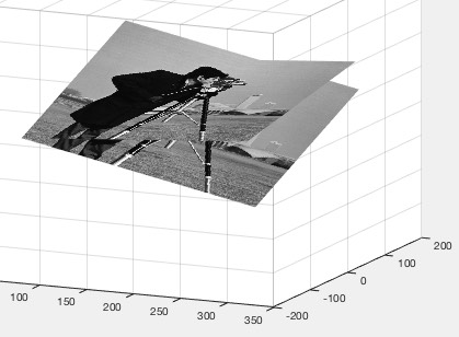 |
% imwarpT(I,T,scal,cent,fc) - warps an image related to a give transformation matrix % (by Tim Lueth, VLFL-Lib, 2017-MAI-10 as class: USER INTERFACE) % % Introduced first in SolidGeometry 3.8 % % See also: VLwarpgrid, warp, imwarp, imageofVLprojection % % h=imwarpT(I,[T,scal,cent,fc]) % === INPUT PARAMETERS === % I: image or image size [r c] % T: Transformation matrix % scal: scaling factor % cent: true if centered; default is false % fc: frame color such as 'b-'; default is ''; % === OUTPUT RESULTS ====== % h: handle to image % % EXAMPLE: % I=imread('cameraman.tif'); % imwarpT(I,TofR(rot(pi/6,pi/6,pi/6))); % imwarpT(I,TofR(rot(pi/6,pi/3,pi/6))); % SGfigure; imwarpT(I,TofR(rot(pi/6,pi/6,pi/6)),[0.1 0.1],true); % SGfigure; imwarpT(I,eye(4),[0.1 0.1],true,'b-'); show % % See also: VLwarpgrid, warp, imwarp, imageofVLprojection % |
VLwarpgrid(siz,T,scal)- creates a meshgrid for warping an image |
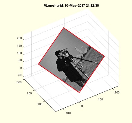 |
% VLwarpgrid(siz,T,scal) - creates a meshgrid for warping an image % (by Tim Lueth, VLFL-Lib, 2017-MAI-10 as class: USER INTERFACE) % % See also: imwarpT % % [VL,XL,YL,ZL]=VLwarpgrid([siz,T,scal]) % === INPUT PARAMETERS === % siz: image or image size [r c] % T: Transformation matrix % scal: scaling factor % === OUTPUT RESULTS ====== % VL: Vertex list % XL: warp grid X % YL: warp grid Y % ZL: warp grid Z % % EXAMPLE: % I=imread('cameraman.tif'); % VLwarpgrid(I,TofR(rot(pi/6,0,0)));; % |
PLofVLprojection(VL,pc,pt,cup,sc,isize)- returns image point on a target screen |
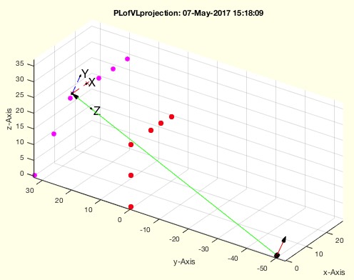 |
% PLofVLprojection(VL,pc,pt,cup,sc,isize) - returns image point on a target screen % (by Tim Lueth, VLFL-Lib, 2017-MAI-07 as class: ANALYTICAL GEOMETRY) % % Fnctn to simulate a c-arm or central projection to a flat screen % (Status of: 2017-05-09) % % See also: TofcamVLPL % % [PL,T,VLT,Tc]=PLofVLprojection([VL,pc,pt,cup,sc,isize]) % === INPUT PARAMETERS === % VL: Vertex list % pc: camera center % pt: target image origin % cup: camera up center; default is [0 0 1] % sc: image scaling (pixel size); default is [1 1] % isize: image size; default is 512 512 % === OUTPUT RESULTS ====== % PL: Point List in image coordinate system % T: T matrix of image coordinate system % VLT: Position of the projektion points in VL's system % Tc: T matrix of camera coordinate system % % EXAMPLE: % PLofVLprojection(VLsample(7),[0 -50 0],[0 20 30],[1 0 0]) % PLofVLprojection(VLsample(7),[0 -50 0],[0 20 30],[0 0 1]) % VL=10*rand(10,3), PLofVLprojection(VL) % |
TofVLprojection()- returns the HT matrix of camera based on a VL and Projection image PL |
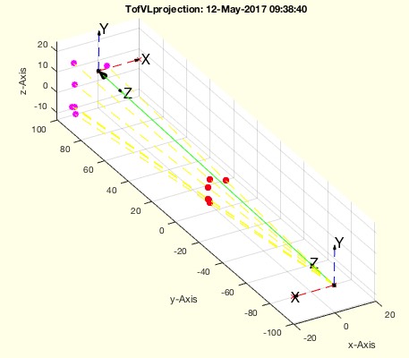 |
% TofVLprojection() - returns the HT matrix of camera based on a VL and Projection image PL % (by Tim Lueth, VLFL-Lib, 2017-MAI-06 as class: ANALYTICAL GEOMETRY) % % ======================================================================= % OBSOLETE (2017-05-12) - USE FAMILY 'TofcamVLPL' INSTEAD % ======================================================================= % % exactly the same as TofcamVLPL (Status of: 2017-05-07) % % [T,K,s,azxz]=TofVLprojection([]) % === OUTPUT RESULTS ====== % T: % K: % s: % azxz: % |
Tofgca- returns the HT matrix of the current camera position |
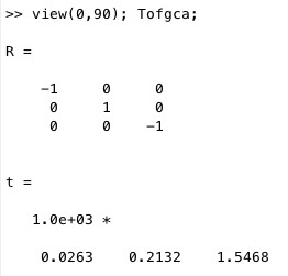 |
% Tofgca - returns the HT matrix of the current camera position % (by Tim Lueth, VLFL-Lib, 2017-MAI-02 as class: ANALYTICAL GEOMETRY) % % Tofgca returns the current axis's camera values as HT Matrix % Tofcam returns either for given or the current axis's camera values as % HT Matrix (Status of: 2017-05-11) % % See also: showcam, Tofcam % % [T,Tt,va,ax]=Tofgca % === OUTPUT RESULTS ====== % T: HT matrix of camera coordinate system % Tt: HT of target coordinate system % va: current camera angle % ax: current camera axis % % EXAMPLE: Just try % SGfigure; SGplot(SGsample(1)); pause (1); Tofgca; pause(1); axis tight; % view(-30,30) % |
showcam- draws a copy of the current figure including the current camera situation |
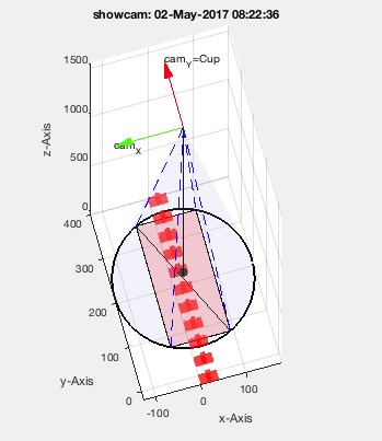 |
% showcam - draws a copy of the current figure including the current camera situation % (by Tim Lueth, VLFL-Lib, 2017-MAI-01 as class: VISUALIZATION) % % See also: Tofgca, camset, campos, camplot % % showcam % % EXAMPLE: % SGfigure; SGmodelOR(1) % showcam % |
exp_2017_05_01- EXPERIMENT that visuaize the current projection situation |
 |
% exp_2017_05_01 - EXPERIMENT that visuaize the current projection situation % (by Tim Lueth, VLFL-Lib, 2017-MAI-01 as class: USER INTERFACE) % % Final fnctn called: showcam (Status of: 2017-05-01) % % See also: camset, camplot % % exp_2017_05_01 % |
SGof2CPLsz(CPA,CPB,z,stype,ctype)- returns a solid defined by 2 contours and height |
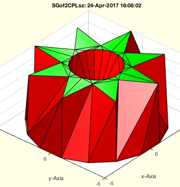 |
% SGof2CPLsz(CPA,CPB,z,stype,ctype) - returns a solid defined by 2 contours and height % (by Tim Lueth, VLFL-Lib, 2017-APR-24 as class: SURFACES) % % This fnctn is the same as SGof2CPLz but supports more than one contour! % The optimal result depends on the expectations of the user. Consider % different options for stype carefully: % "number" of points, i.e. 1:nmax % "length" of contour, i.e. 0:sum(edge length) % "angle" of contour, i.e. 0:sum(abs(edge angle)) % "center" of contour, i.e. 0:360 degree % also the starting point ctype ('rot' or 'min'); % Quite optimal procedure to find the walls between two planar contours % without adding new points. The number of faces is na+nb. % The resulting vertex list SG: % SG.VL=[VLaddz(CPA,0);VLaddz(CPB,z)]; % SG.FL=[FLA;FLB;FLW]; % (Status of: 2017-06-12) % % Introduced first in SolidGeometry 3.8 % % See also: SGof2SGT, SGof2T, SGof2CVL, SGof2CPLz, SGofCPLzchamfer, % SGof2CPLzheurist, SGof2CPLzbranch % % [SG,FLW,FLA,FLB]=SGof2CPLsz([CPA,CPB,z,stype,ctype]) % === INPUT PARAMETERS === % CPA: ONE bottom Contour % CPB: ONE top Contour % z: height of the solid % stype: "number", "length", "angle", "center"; default is "length" % ctype: "rot" or "miny"; default is "rot" % === OUTPUT RESULTS ====== % SG: Solid Geoemtry; VL=[CPA;CPB] % FLW: Face list of Wall % FLA: Face list of CPA % FLB: Face list of CPB % % EXAMPLE: % CPA=[PLcircle(5.1,16);NaN NaN; PLcircle(2,4)]; % CPB=[PLstar(5,16,[],[],[],0.5);NaN NaN; PLcircle(2)]; % SGof2CPLsz(CPA,CPB,5) % % See also: SGof2SGT, SGof2T, SGof2CVL, SGof2CPLz, SGofCPLzchamfer, % SGof2CPLzheurist, SGof2CPLzbranch % |
exp_2017_04_24- EXPERIMENT to create drawing templates with prismatic angles => |
 |
% exp_2017_04_24 - EXPERIMENT to create drawing templates with prismatic angles => % (by Tim Lueth, VLFL-Lib, 2017-APR-24 as class: EXPERIMENTS) % % EXPERIMENT to create a fnctn for drawing templates (Zeichen schablone) % Resulting fnctns are % 1. SGof2CPLsz % (Status of: 2017-04-24) % % exp_2017_04_24 % |
BBofCPL(CPL)- returns the bounding box of a CPL |
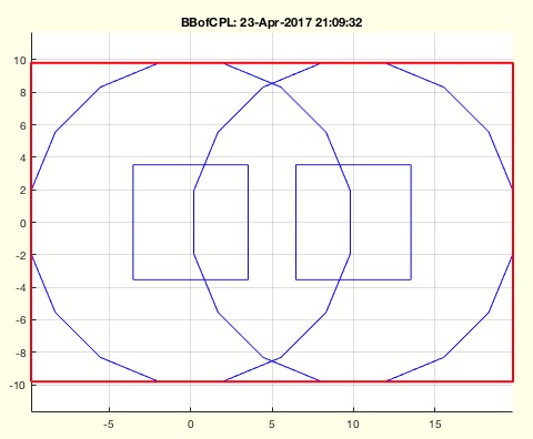 |
% BBofCPL(CPL) - returns the bounding box of a CPL % (by Tim Lueth, VLFL-Lib, 2017-APR-23 as class: CLOSED POLYGON LISTS) % % See also: CPLofBB, BBofVL, BBofSG % % bb=BBofCPL(CPL) % === INPUT PARAMETERS === % CPL: Closed Polygon Line % === OUTPUT RESULTS ====== % bb: bb [xmin xmax ymin ymax] % |
CPLofmeshgrid(X,Y)- returns two grid line templates |
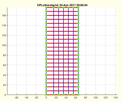 |
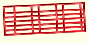
% CPLofmeshgrid(X,Y) - returns two grid line templates % (by Tim Lueth, VLFL-Lib, 2017-APR-23 as class: CLOSED POLYGON LISTS) % % See also: CPLof % % [CPL,PLX,PLY,PL]=CPLofmeshgrid(X,Y) % === INPUT PARAMETERS === % X: List of X values % Y: List of Y values % === OUTPUT RESULTS ====== % CPL: Complete list of lines % PLX: Only X lines % PLY: Only Y lines % PL: Point List (unique) % % EXAMPLE: % CPLtemplateofCPL(CPLofmeshgrid([0 15 25 35 45 55 65],0:8:8*22),1,true); % SGdrawingtemplateofCPL(CPLofmeshgrid([0 15 25 35 45 55 65],8*[0 1 6 8 % 13 15 20 23]),1) % SGdrawingtemplateofCPL(B,1) % |
CPLunitesorted(CPL)- returns sorted and added closed polygons |
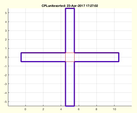 |
% CPLunitesorted(CPL) - returns sorted and added closed polygons % (by Tim Lueth, VLFL-Lib, 2017-APR-23 as class: CLOSED POLYGON LISTS) % % ..have the impression to have implemented this fnctn already several % times in different manner.. (Status of: 2017-04-23) % % See also: CPLsortinout, CPLpolybool % % CPLN=CPLunitesorted(CPL) % === INPUT PARAMETERS === % CPL: Closed Polygon Line % === OUTPUT RESULTS ====== % CPLN: systematically ordered and Boolean operated CPL % % EXAMPLE: % A=[0 0; 10 0;NaN NaN;5 -5; 5 +5] % CPLunitesorted(CPLtemplateofCPL(A)) % |
CPLtemplateofCPL(CPL,pen,un)- returns a template for a given CPL |
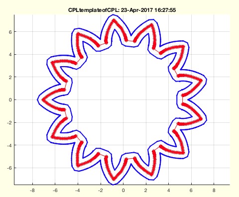 |
% CPLtemplateofCPL(CPL,pen,un) - returns a template for a given CPL % (by Tim Lueth, VLFL-Lib, 2017-APR-23 as class: CLOSED POLYGON LISTS) % % Attention: This fnctn distinguishs between open and closed PL / CPLs % for obvious reasons. Threfor close a PL such as PLcircle or PLstar by % CPLofPL. (Status of: 2017-04-23) % % Introduced first in SolidGeometry 3.8 % % See also: CPLgrow, PLgrow % % CPN=CPLtemplateofCPL(CPL,[pen,un]) % === INPUT PARAMETERS === % CPL: CPL separated by NaN NaN % pen: diameter of template % un: if true; contours are united; default is false; % === OUTPUT RESULTS ====== % CPN: % % EXAMPLE: % A=[0 0; 10 0;NaN NaN;5 -5; 5 +5]; CPLtemplateofCPL(A,2,false) % A=[0 0; 10 0;NaN NaN;5 -5; 5 +5]; CPLtemplateofCPL(A,2,true) % CPLtemplateofCPL(PLsample(1)) % CPLtemplateofCPL(PLsample(2)) % CPLtemplateofCPL(PLsample(11),12) % CPLtemplateofCPL(CPLoftext('s')) % CPLtemplateofCPL(PLgearDIN(1,13)) % % See also: CPLgrow, PLgrow % |
PLsample(n)- returns a 2D PL list similar to VLsample |
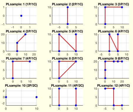 |
% PLsample(n) - returns a 2D PL list similar to VLsample % (by Tim Lueth, VLFL-Lib, 2017-APR-23 as class: ANALYTICAL GEOMETRY) % % For many fnctns it is helpful to have a sample point list (Status of: % 2017-07-16) % % Introduced first in SolidGeometry 3.8 % % See also: CPLsample, VLsample, SGsample, CPLoftext, VLFLsample % % PL=PLsample([n]) % === INPUT PARAMETERS === % n: sample of Point List % === OUTPUT RESULTS ====== % PL: returns PL if n>0 % % See also: CPLsample, VLsample, SGsample, CPLoftext, VLFLsample % |
SGdrawingtemplateofCPL(CPLU,pen,unt,wall,height,dmin,lnk,top)- Creates a 3D printable drawing template - slow but helpful |
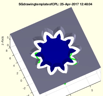 |
% SGdrawingtemplateofCPL(CPLU,pen,unt,wall,height,dmin,lnk,top) - Creates a 3D printable drawing template - slow but helpful % (by Tim Lueth, VLFL-Lib, 2017-APR-23 as class: MODELING PROCEDURES) % % When creating templates from a line drawing, a contour is moved % outwards and inwards: CPLgrow. This can lead to self-overlaps of % contours. Accordingly, the out-contour of the grown contour and the % inner contour of the fringed contour must be used: CPLsortinout. The % fnctn is: CPLtemplateofCPL. Insulated contours are then connected: % CPLunitesorted. Overlapping contours are preserved by auxiliary points. % (Status of: 2017-04-25) % % Introduced first in SolidGeometry 3.8 % % See also: CPLtemplateofCPL % % SG=SGdrawingtemplateofCPL(CPLU,[pen,unt,wall,height,dmin,lnk,top]) % === INPUT PARAMETERS === % CPLU: Linienzeichnung % pen: pen diameter % unt: if true; crossings are united; default is false % wall: wall thickness; default is 1.5mm % height: height of template; default is 1.5mm % dmin: diameter to support crossing points % lnk: if true, solids are connected; default is false % top: upper pen diameter; default is width; % === OUTPUT RESULTS ====== % SG: SG of a drawing template % % EXAMPLE: % A=[0 0; 10 0;NaN NaN;5 -5; 5 +5]; SGdrawingtemplateofCPL(A,1,false); % A=[0 0; 10 0;NaN NaN;5 -5; 5 +5]; SGdrawingtemplateofCPL(A,1,true); % SGdrawingtemplateofCPL([0 0; 10 0]) % SGdrawingtemplateofCPL(PLgearDIN(1,10)) % % See also: CPLtemplateofCPL % |
PLsplitpointsofCPL(CPL)- returns splitpoints created by delaunaytriangulation |
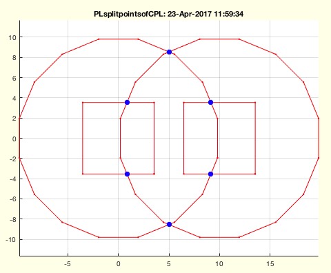 |
% PLsplitpointsofCPL(CPL) - returns splitpoints created by delaunaytriangulation % (by Tim Lueth, VLFL-Lib, 2017-APR-23 as class: CLOSED POLYGON LISTS) % % Introduced first in SolidGeometry 3.8 % % See also: CPLsplitpoints % % SPL=PLsplitpointsofCPL(CPL) % === INPUT PARAMETERS === % CPL: CPL separated by NaN % === OUTPUT RESULTS ====== % SPL: List of splitpoints created by delaunaytriangulation % % EXAMPLE: % PLsplitpointsofCPL(CPLsample(16)) % % See also: CPLsplitpoints % |
SGcopyVL(SG,VL,fuse)- returns a cell list of copies of SG an positions of VL |
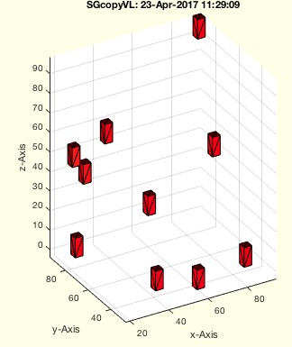 |
% SGcopyVL(SG,VL,fuse) - returns a cell list of copies of SG an positions of VL % (by Tim Lueth, VLFL-Lib, 2017-APR-23 as class: SURFACES) % % Introduced first in SolidGeometry 3.8 % % See also: SGarrangeSG, SGcopyrotZ % % SGC=SGcopyVL(SG,VL,[fuse]) % === INPUT PARAMETERS === % SG: Solid Geometry % VL: Coordiantes for creating a copy of SG % fuse: if true; SG is struct not cell; default is true % === OUTPUT RESULTS ====== % SGC: cell list of SG % % EXAMPLE: Create copies at ten random positions % SGcopyVL(SGbox([4,4,10]),100*rand(10,3)) % % See also: SGarrangeSG, SGcopyrotZ % |
lastwarnTL- returns information on the last warnings |
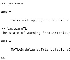 |
% lastwarnTL - returns information on the last warnings % (by Tim Lueth, VLFL-Lib, 2017-APR-23 as class: AUXILIARY PROCEDURES) % % For a programmer, who wants to know which warning should be switched % off, the sequence of lastwarn is may not optimal; should be flipped % (Status of: 2017-07-15) % % Introduced first in SolidGeometry 3.8 % % See also: lastwarnoff, lastwarn % % [b,a]=lastwarnTL % === OUTPUT RESULTS ====== % b: LASTID % a: LASTMSG % % EXAMPLE: % lastwarnTL % warning('off','last'); % % % See also: lastwarnoff, lastwarn % |
ginput2Dcircle(gr,ax)- returns by user interaction center and radius of a circle |
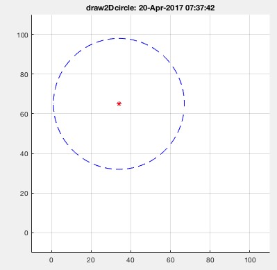 |
% ginput2Dcircle(gr,ax) - returns by user interaction center and radius of a circle % (by Tim Lueth, VLFL-Lib, 2017-APR-20 as class: USER INTERFACE) % % Introduced first in SolidGeometry 3.8 % % [cc,cr,h]=ginput2Dcircle([gr,ax]) % === INPUT PARAMETERS === % gr: grid resolution; default is 1 % ax: axis of the screen; default is % === OUTPUT RESULTS ====== % cc: center of circle % cr: radius of circle % h: % |
SGofpatch(gh,fuse)- returns a SG from a patch |
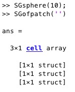 |
% SGofpatch(gh,fuse) - returns a SG from a patch % (by Tim Lueth, VLFL-Lib, 2017-APR-19 as class: SURFACES) % % See also: patchofSG, SGplot, reducepatch, reducepatchSG % % SG=SGofpatch([gh,fuse]) % === INPUT PARAMETERS === % gh: handle to patch; default is patchofgca % fuse: if true; create only one SG; default is false; % === OUTPUT RESULTS ====== % SG: Solid Geoemtry; single or cells % |
patchofSG(SG,realp)- creates a patch struct of a solid geometry |
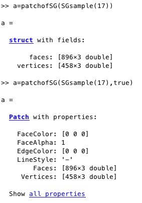 |
% patchofSG(SG,realp) - creates a patch struct of a solid geometry % (by Tim Lueth, VLFL-Lib, 2017-APR-19 as class: USER INTERFACE) % % Matlab has different data models for the handling of surface models: % patch, triangulation, delaunaytriangulation, poly2fv etc. % SUPPORTS also with cells of solids an returns a list % ATTENTION: A patch is only valid if the figure is not closed. So in % case that you want to use a patch for surface reduction, copy it % afterwards into a SG using 'SGofpatch'; It is similar to SGplot (Status % of: 2017-06-17) % % See also: SGofpatch, SGplot, SGreduceVLFL % % h=patchofSG(SG,[realp]) % === INPUT PARAMETERS === % SG: Soldid Geometry; % realp: true=real patch; default is false % === OUTPUT RESULTS ====== % h: handle to patch struct or patch class % % EXAMPLE: % a=patchofSG(SGsample(17)) % a=patchofSG(SGsample(17),true) % |
patchofgca(gh)- returns all patches of the current graphics axis |
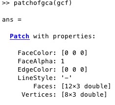 |
% patchofgca(gh) - returns all patches of the current graphics axis % (by Tim Lueth, VLFL-Lib, 2017-APR-19 as class: USER INTERFACE) % % simple macro: h=findall(gh,'type','patch'); (Status of: 2017-04-19) % % See also: SGofpatch, patchofSG, SGplot, reducepatch % % h=patchofgca([gh]) % === INPUT PARAMETERS === % gh: gca or gcf; default gca % === OUTPUT RESULTS ====== % h: handle / handle array % |
reducepatchSG(h,f)- reduces either one or all patches of the current axis |
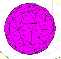 |
% reducepatchSG(h,f) - reduces either one or all patches of the current axis % (by Tim Lueth, VLFL-Lib, 2017-APR-18 as class: SURFACES) % % ======================================================================= % OBSOLETE (2017-06-17) - USE FAMILY 'SGreduceVLFL' INSTEAD % ======================================================================= % % exactly the same as reducepatch, but works with several path arrays and % has default values (Status of: 2017-06-16) % % See also: [ SGreduceVLFL ] ; reducepatch, daspect % % h=reducepatchSG([h,f]) % === INPUT PARAMETERS === % h: handle; default is findall(gca,'type','patch') or SG % f: reduction factor; default is 0.5 % === OUTPUT RESULTS ====== % h: handle or list of handle of gca or SG % % EXAMPLE: % SGsphere(10); reducepatchSG('',0.1); show % SGsphere(10); reducepatchSG('',500); show % SGbox([30,20,10]); pause(1); reducepatchSG('',0.5); show % |
SGofVMisosurface(V,vs,cl)- returns a surface model by the marching cubes |
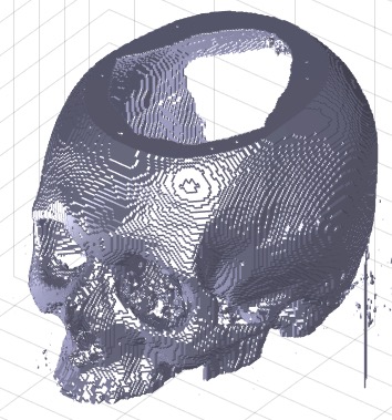 |
% SGofVMisosurface(V,vs,cl) - returns a surface model by the marching cubes % (by Tim Lueth, VLFL-Lib, 2017-APR-18 as class: VOXELS) % % This fnctn is an original Matlab fnctn just a little bit modified to % close surfaces. The fnctn is very similar of SGofVMmarchcube but % definitely slower. Main problem is the unclear method that is % implemented by Matlab. (Status of: 2017-04-18) % % Introduced first in SolidGeometry 3.8 % % See also: VLFLofVMdelaunay, VLFLofVMmarchcube, TR3ofVM, % SGofVMmarchcube, SGofVMdelaunay % % SG=SGofVMisosurface(V,[vs,cl]) % === INPUT PARAMETERS === % V: Logical Volume Model % vs: voxel size, optional % cl: closes open facets by adding empty planes; default is true % === OUTPUT RESULTS ====== % SG: Vertex list % % EXAMPLE: [V,vs]=VMreaddicomdir('AIM_DICOMFILES'); % [a,as]=VMresize(V,[0.5 0.5 0.5],vs); % SG=SGofVMisosurface(a>1400,as); % SGcut(SG,40); % c=CPLofSGslice3(SG,20); % PLFLofCPLdelaunay(c); % PLFLofCPLpoly(c) % % See also: VLFLofVMdelaunay, VLFLofVMmarchcube, TR3ofVM, % SGofVMmarchcube, SGofVMdelaunay % |
isatleastVer(name,TB)- checks the minimal version/release number of matlab |
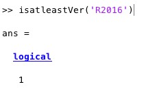 |
% isatleastVer(name,TB) - checks the minimal version/release number of matlab % (by Tim Lueth, VLFL-Lib, 2017-APR-18 as class: AUXILIARY PROCEDURES) % % Introduced first in SolidGeometry 3.8 % % See also: verTL % % is=isatleastVer(name,[TB]) % === INPUT PARAMETERS === % name: Release name 'R2017a' % TB: Toolbox name ;default is 'Matlab' % === OUTPUT RESULTS ====== % is: true or false % % EXAMPLE: % isatleastVer('R2017b') % isatleastVer('R2017a') % % See also: verTL % |
verTL(name)- returns the currently used Matlab Release |
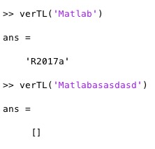 |
% verTL(name) - returns the currently used Matlab Release % (by Tim Lueth, VLFL-Lib, 2017-APR-18 as class: AUXILIARY PROCEDURES) % % More simple to use than 'ver' (Status of: 2017-07-07) % % Introduced first in SolidGeometry 3.8 % % See also: ver, isatleastVer % % v=verTL(name) % === INPUT PARAMETERS === % name: Tool to search for % === OUTPUT RESULTS ====== % v: RElease such as 'R2017a'; empty if missing; % % EXAMPLE: % ver % verTL('Matlab') % verTL('Matlabasasdasd') % verTL('Mapping Toolbox') % % % See also: ver, isatleastVer % |
VMwindowplot(V,cax,minv,maxv)- plots a voxel model using the window caxis function |
 |
% VMwindowplot(V,cax,minv,maxv) - plots a voxel model using the window caxis fnctn % (by Tim Lueth, VLFL-Lib, 2017-APR-12 as class: VOXELS) % % shows only the voxels within the specified intensity interval and voxel % intervall (Status of: 2017-04-17) % % See also: VMplot, VMcaxis % % VX=VMwindowplot(V,[cax,minv,maxv]) % === INPUT PARAMETERS === % V: Voxel model % cax: [cmin cmax]; % minv: minimum voxel value; values <0 are precentage % maxv: maximum voxel value; values <0 are precentage % === OUTPUT RESULTS ====== % VX: % % EXAMPLE: % VMwindowplot(V,[400 1200],0.2,0.7); % SGofVMmarchcube(VX) % |
VMcaxis (cax)- adjustes the caxis of the VMplot diagram |
 |
% VMcaxis (cax) - adjustes the caxis of the VMplot diagram % (by Tim Lueth, VLFL-Lib, 2017-APR-12 as class: VOXELS) % % VMcaxis([cax]) % === INPUT PARAMETERS === % cax: [cmin cmax]; default is min and max of the current! surfaces % |
numofstrtab(tok,strtab)- returns a row number of a cell list of strings |
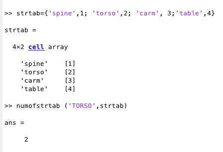 |
% numofstrtab(tok,strtab) - returns a row number of a cell list of strings % (by Tim Lueth, VLFL-Lib, 2017-APR-09 as class: AUXILIARY PROCEDURES) % % See also: SGmodelOR % % nr=numofstrtab(tok,strtab) % === INPUT PARAMETERS === % tok: string to compare with; % strtab: cell list; frist col = string % === OUTPUT RESULTS ====== % nr: cell list row, col 2: end % % EXAMPLE: % strtab={'spine',1; 'torso',2; 'carm', 3;'table',4}; % numofstrtab ('TORSO',strtab); % |
SGmodelOR(part)- returns solid model of OR device models |
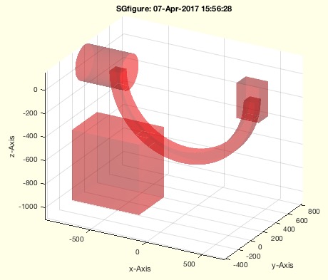 |
% SGmodelOR(part) - returns solid model of OR device models % (by Tim Lueth, VLFL-Lib, 2017-APR-07 as class: SURFACES) % % The following (Status of: 2017-04-17) % % Introduced first in SolidGeometry 3.8 % % See also: SGsample, CPLsample, VLSample % % SG=SGmodelOR(part) % === INPUT PARAMETERS === % part: % === OUTPUT RESULTS ====== % SG: Solid geometry of part % % See also: SGsample, CPLsample, VLSample % |
CELofEL(EL)- returns a corrected succeding EL for a single contour |
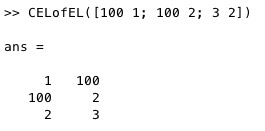 |
% CELofEL(EL) - returns a corrected succeding EL for a single contour % (by Tim Lueth, VLFL-Lib, 2017-APR-07 as class: EDGE LISTS) % % branches are not alloweed, i.e. % - two terminals and m links % - or n links (Status of: 2017-04-07) % % See also: treeNodesofEL % % [CEL,CHN]=CELofEL(EL) % === INPUT PARAMETERS === % EL: unsorted but correct edge list % === OUTPUT RESULTS ====== % CEL: Sorted Edge list of Contour or Line of Nodes % CHN: Chain [n x 1] with nodes % % EXAMPLE: % CELofEL([100 1; 100 2; 3 2; 1 3]) % |
ELsort(EIL)- returns a increasing sorted edge list separated by NaN |
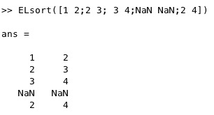 |
% ELsort(EIL) - returns a increasing sorted edge list separated by NaN % (by Tim Lueth, VLFL-Lib, 2017-APR-06 as class: AUXILIARY PROCEDURES) % % Does replace sortEL. Branches are not allowed! Use % This fnctn is able to handle NaN separated Edge lists and orders them % upwards from frist to last and left to right. In addition the chains % are linked together % woNaN can be used ti remove the NaN NaN separators later. (Status of: % 2017-04-07) % % See also: ELunsort, ELuniqueofFL, CELofEL, woNaN % % EIL=ELsort(EIL) % === INPUT PARAMETERS === % EIL: Edge List % === OUTPUT RESULTS ====== % EIL: Edge List % |
treeNodesofEL(EL)- returns the tree structure from a given edge list |
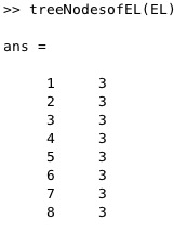 |
% treeNodesofEL(EL) - returns the tree structure from a given edge list % (by Tim Lueth, VLFL-Lib, 2017-APR-06 as class: EDGE LISTS) % % Fnctn removes lines with Nan first: In a list there are: % - single used points (Terminals) % - doubled used points (Links) % - three or more times used points (Branches) % (Status of: 2017-04-07) % % See also: CELofEL % % [vi,vc,bi,ti,li]=treeNodesofEL(EL) % === INPUT PARAMETERS === % EL: Edge list % === OUTPUT RESULTS ====== % vi: list of vertices [vi n] % vc: vertes use counter [bi ti li] % bi: branch index % ti: terminal index % li: link index % % EXAMPLE: % A=SGbox([30,20,10]); EL=FEofSG(A); treeNodesofEL(EL) % |
VLremsuccident(VL)- removes succeding identical rows in a list |
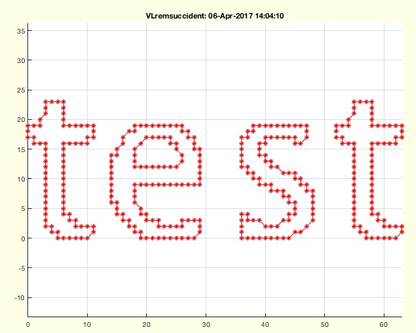 |
% VLremsuccident(VL) - removes succeding identical rows in a list % (by Tim Lueth, VLFL-Lib, 2017-APR-06 as class: AUXILIARY PROCEDURES) % % Fnctn is able to handle doubled nan too! It was designed for open PL % ways returns a PL/VL since last and frist point are succeeding points % and the first remains. (Status of: 2017-04-07) % % Introduced first in SolidGeometry 3.8 % % See also: CVLremstraight % % [SVL,ii]=VLremsuccident(VL) % === INPUT PARAMETERS === % VL: list of numeric rows % === OUTPUT RESULTS ====== % SVL: decimated list % ii: removed indices in original list % % EXAMPLE: % CPL=roundn(CPLaddauxpoints(CPLoftext('test'),1),1) % VLremsuccident(CPL) % % See also: CVLremstraight % |
CVLremstraight (CVL,de,al)- returns straight points on a line depending on distance and agle |
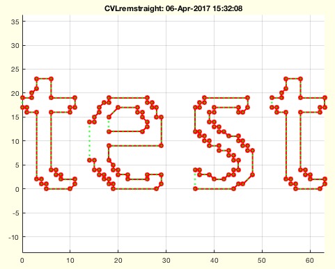 |
% CVLremstraight (CVL,de,al) - returns straight points on a line depending on distance and agle % (by Tim Lueth, VLFL-Lib, 2017-APR-06 as class: ANALYTICAL GEOMETRY) % % able to handel CPL % checks identical points (1),(end) % removes identical succeeding points % removes points neadby % removes angle points less than one degree (Status of: 2017-04-06) % % Introduced first in SolidGeometry 3.8 % % See also: VLremsuccident % % CVLremstraight(CVL,[de,al]) % === INPUT PARAMETERS === % CVL: Contour verteex list % de: default is 1e-6; % al: default is 1 degree % % EXAMPLE: % CPL=roundn(CPLaddauxpoints(CPLoftext('test'),1),1) % CVLremstraight(CPL) % % See also: VLremsuccident % |
FEofSG(SG,ang)- returns FE and optional VL of a solid geometry or of gca |
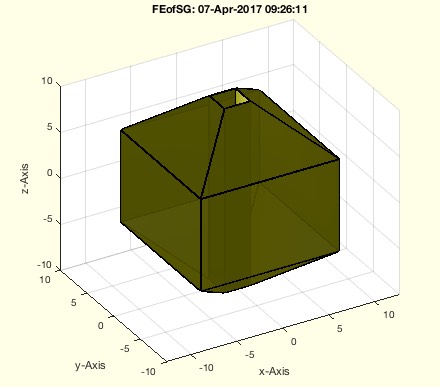 |
% FEofSG(SG,ang) - returns FE and optional VL of a solid geometry or of gca % (by Tim Lueth, VLFL-Lib, 2017-APR-06 as class: SURFACES) % % Introduced first in SolidGeometry 3.8 % % See also: VLFLofgca, FEplot % % [FE,VL]=FEofSG([SG,ang]) % === INPUT PARAMETERS === % SG: if empty; VLFLofgca is used % ang: angle; default is 0.4 ~ pi/8 % === OUTPUT RESULTS ====== % FE: Feature edge list % VL: Vertex list for embedded SG % % EXAMPLE: % FEofSG(SGsample(3)) % % See also: VLFLofgca, FEplot % |
viewdimensioning(a,b,crossp,alpha)- changes the view parameter for an engineering view |
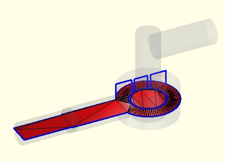 |
% viewdimensioning(a,b,crossp,alpha) - changes the view parameter for an engineering view % (by Tim Lueth, VLFL-Lib, 2017-APR-05 as class: USER INTERFACE) % % This fnctn works similar to view but allows to add a crossing point to % see only a crossing plane; % Nevertheless such a crossing plane requires in fact a real slicing of % the sold at the right possition (Status of: 2017-04-17) % % Introduced first in SolidGeometry 3.8 % % See also: view, PLdimensioning, CVLdimclassifier % % % [CPL,CVL,X]=viewdimensioning([a,b,crossp,alpha]) % === INPUT PARAMETERS === % a: view angle a % b: view angle b % crossp: optional crossing point / plane % alpha: alpha value % === OUTPUT RESULTS ====== % CPL: Contour Point list x y 0 % CVL: Contour vertex list x y z % X: Crossing Solid % % EXAMPLE: % SGfigure(SGsample(17)); CPL=viewdimensioning(0,0,[0 0 0]); % PLdimensioning(CPL); % SGfigure(SGsample(17)); CPL=viewdimensioning(-90,0,[0 0 0]); % PLdimensioning(CPL); % % close all; SGfigure(SGsample(17)); view(-30,30); % view(0,90) % viewdimensioning(0,-90,[0 0 15],0.1) % [a,b,c]=viewdimensioning(0,-90,[0 0 15],0.1); % SGplot(c); CVLplot(b,'b-',3); % % See also: view, PLdimensioning, CVLdimclassifier % % |
CVLdimclassifier(OVL)- analyses contours and classifies different drawing elements |
 |
% CVLdimclassifier(OVL) - analyses contours and classifies different drawing elements % (by Tim Lueth, VLFL-Lib, 2017-APR-04 as class: USER INTERFACE) % % This fnctn returns simple points that should be dimensioned. They do % not specify a contour. In addition the fnctn also returns a list of % radial centers and radius % [cx cy cz] is the center of a circle; % deg is the length of the circle % (Status of: 2017-06-25) % % Introduced first in SolidGeometry 3.8 % % See also: PLdimensioning % % [DVL,RL,RIL,Rnv]=CVLdimclassifier(OVL) % === INPUT PARAMETERS === % OVL: Contour vertex List % === OUTPUT RESULTS ====== % DVL: List for dimensioning % RL: [cx cy cz Nr deg R vx vy vz] % RIL: Points % Rnv: List of normal vectors related to RL % % EXAMPLE: % CVLdimclassifier(PLradialEdges(CPLofPL(PLsquare(30,20)),4)); % % % See also: PLdimensioning % |
expname(pfix)- returns a filename with the current date |
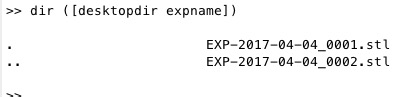 |
% expname(pfix) - returns a filename with the current date % (by Tim Lueth, VLFL-Lib, 2017-APR-04 as class: FILE HANDLING) % % Introduced first in SolidGeometry 3.8 % % See also: desktopdir, pcodedirTL, smbFilename, smbPSLibname % % fname=expname([pfix]) % === INPUT PARAMETERS === % pfix: prefix default is 'EXP-' % === OUTPUT RESULTS ====== % fname: file or directory name % % EXAMPLE: % dir ([desktopdir expname]) % % See also: desktopdir, pcodedirTL, smbFilename, smbPSLibname % |
PLdimensioning(CPL)- plots a measurement ruler under a CPL |
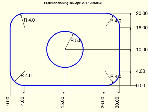 |
% PLdimensioning(CPL) - plots a measurement ruler under a CPL % (by Tim Lueth, VLFL-Lib, 2017-APR-04 as class: USER INTERFACE) % % WORK in progress. Does support % - removal of points on straight lines % - holes and radial corners % (Status of: 2017-04-17) % % Introduced first in SolidGeometry 3.8 % % See also: CPLsortinout, CVLdimclassifier, view, viewdimensioning % % h=PLdimensioning(CPL) % === INPUT PARAMETERS === % CPL: CPL or PL % === OUTPUT RESULTS ====== % h: handle to drawings % % EXAMPLE: % PLdimensioning(CPLsample(3)); % PLdimensioning(CPLofPL(PLradialEdges(PLsquare(30,20),4))); % PLdimensioning(CPLofPL(PLradialEdges(CPLofPL(PLsquare(30,20)),4))); % PLdimensioning([CPLofPL(PLradialEdges(CPLofPL(PLsquare(30,20)),4));NaN % NaN;PLcircle(5)]); % % See also: CPLsortinout, CVLdimclassifier, view, viewdimensioning % |
SGsurfacehistogram(B,si,be)- plots a surface area histogram of selected surfaces |
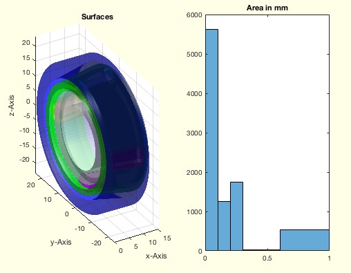 |
% SGsurfacehistogram(B,si,be) - plots a surface area histogram of selected surfaces % (by Tim Lueth, VLFL-Lib, 2017-APR-04 as class: SURFACES) % % This fnctn is useful to analyze imported STL files generated by a CSG % modeler such as Catia. % Rounded edges or broken corners makes it difficult to analyze fnctnal % surface manually. This fnctn helps to get a feeling for the CSG-to-STL % conversion strategy. (Status of: 2017-04-04) % % Introduced first in SolidGeometry 3.8 % % See also: SGsurfaceplot, SGsurfaces % % SGsurfacehistogram(B,[si,be]) % === INPUT PARAMETERS === % B: Solid Geoemtry % si: surface index wrt SGsurfaces; default '' % be: histogram bin edges; default is be=[0 0.1 0.2 0.3 0.4 0.5 0.6 1.0]; % % % EXAMPLE: % SGsurfacehistogram(SGsample(17)) % SGsurfacehistogram(SGsample(17),'',1:10) % % See also: SGsurfaceplot, SGsurfaces % |
SGisconvex(SG)- returns whether a solid is convex |
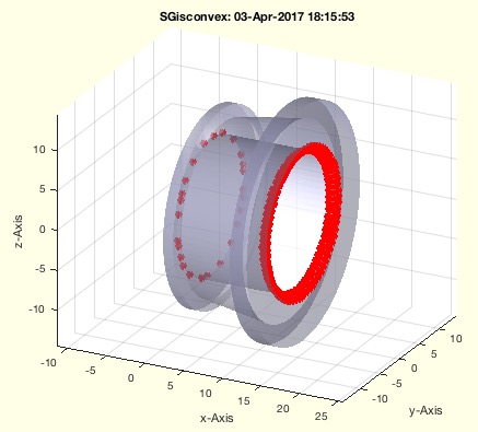 |
% SGisconvex(SG) - returns whether a solid is convex % (by Tim Lueth & Felix Schoppa, VLFL-Lib, 2017-APR-03 as class: SURFACES) % % WORK IN PROGRESS (2017-04-03) % A solid is convex if all normal vectors of the vertices have the same % direction, i.e.if the angle between vector from center line to vertex % and verte normal vector is less than 90 degree (pi/2); % (Status of: 2017-04-03) % % c=SGisconvex(SG) % === INPUT PARAMETERS === % SG: Solid Geometry % === OUTPUT RESULTS ====== % c: true if convex, false if not % |
SGsurfaces(SG,slct)- returns a cell list of separated CLOSED surfaces similar to SGseparate |
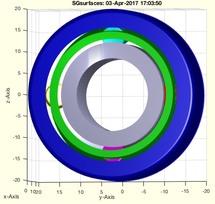 |
% SGsurfaces(SG,slct) - returns a cell list of separated CLOSED surfaces similar to SGseparate % (by Tim Lueth, VLFL-Lib, 2017-APR-03 as class: SURFACES) % % SGsurfaces and SGseparate analyse independent closed surfaces. % SGanalyzeGroupParts analyses penetration of surfaces. % For open surfaces use surfacesofSG (Status of: 2017-07-07) % % Introduced first in SolidGeometry 3.8 % % See also: SGsurfaceplot, SGsurfacehistogram, SGseparate, SGpacking, % SGwriteSeparatedSTL, SGanalyzeGroupParts, surfacesofSG % % [SGC,n]=SGsurfaces(SG,[slct]) % === INPUT PARAMETERS === % SG: Solid geoemtry as single struct % slct: surface index; default is all; SGseparate shows all % === OUTPUT RESULTS ====== % SGC: cell list of solid geometry structs % n: length of cell list % % EXAMPLE: % SGsurfaces(SGsample(17)) % SGwriteSeparatedSTL(SGsurfaces(SGsample(17))) % SGpacking(SGsurfaces(SGsample(17))) % % See also: SGsurfaceplot, SGsurfacehistogram, SGseparate, SGpacking, % SGwriteSeparatedSTL, SGanalyzeGroupParts, surfacesofSG % |
VMintensityscale(V,cax)- returns an intensity scaled voxel image |
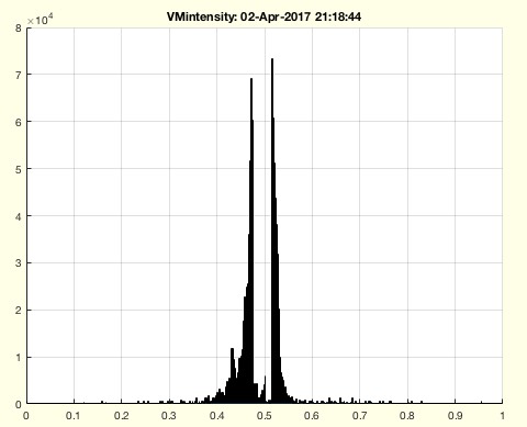 |
% VMintensityscale(V,cax) - returns an intensity scaled voxel image % (by Tim Lueth, VLFL-Lib, 2017-APR-02 as class: VOXELS) % % See also: VMplot, VMmontage, VMresize % % [c,V]=VMintensityscale(V,[cax]) % === INPUT PARAMETERS === % V: Voxel mode % cax: desired intensity interval; default is [0 1] % === OUTPUT RESULTS ====== % c: [minc maxc] % V: scaled to 0 to 1 % |
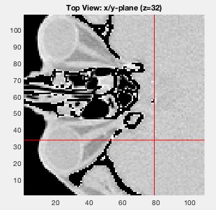
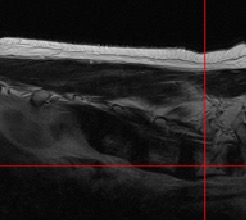
getprojectionimage(pc,vdist,vwidth,cupv)- returns a single projection image of gca |
 |
% getprojectionimage(pc,vdist,vwidth,cupv) - returns a single projection image of gca % (by Tim Lueth, VLFL-Lib, 2017-APR-02 as class: ANALYTICAL GEOMETRY) % % See also: getgcapixelsize, projectionimage % % I=getprojectionimage(pc,vdist,vwidth,cupv) % === INPUT PARAMETERS === % pc: camera position [-x y z] with direction through [0 0 0] % vdist: distance of the screen behind [0 0 0] % vwidth: length of the screen in y and z % cupv: camera up vector; default is [0 -1 0] % === OUTPUT RESULTS ====== % I: Image calculated by getframe and getgcapixelsize % |
getgcapixelsize- returns the position of the gca in the current figure |
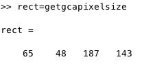 |
% getgcapixelsize - returns the position of the gca in the current figure % (by Tim Lueth, VLFL-Lib, 2017-APR-02 as class: USER INTERFACE) % % This fnctn is required if getframe(gca) does not work anymore. % In this case try getframe(gcf,getgcapixelsize) (Status of: 2017-04-02) % % See also: setgcapixelsize % % rect=getgcapixelsize % === OUTPUT RESULTS ====== % rect: [left bottom width height] in pixels % % EXAMPLE: % subplot(2,2,2) % rect=getgcapixelsize % I=getframe(gcf,rect); figure(3333); imshow(I.cdata); % |
projectionimage(pc,vdist,vwidth,pixel,w)- returns a central projection image by using Matlabs view commands |
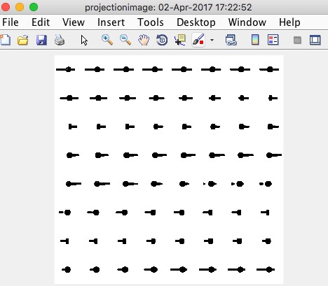 |
% projectionimage(pc,vdist,vwidth,pixel,w) - returns a central projection image by using Matlabs view commands % (by Tim Lueth, Video-Lib, 2017-APR-02 as class: ANALYTICAL GEOMETRY) % % this fnctn returns a projection image of the current gca. The % projections is always done in relation to the point [0 0 0]; The target % is always % % It changes a lot of view parameter such as lighting shading etc. % It can be used to create virtual conebeam images (Status of: 2017-04-02) % % See also: setgcapixelsize, VLprojection % % [I,cax,pc]=projectionimage(pc,vdist,vwidth,[pixel,w]) % === INPUT PARAMETERS === % pc: camera view point % vdist: camera target point % vwidth: virtual screen width % pixel: pixel size of virtual screen % w: single angle value or list an angles; default is 0 % === OUTPUT RESULTS ====== % I: Image of pixel size or image stack % cax: color axis [min max] % pc: center point or list of center points % % EXAMPLE: % SGfigure; SGsample(17); view(-30,30); % projectionimage([0 0 -10],10,200,512,0:pi/32:2*pi-1e-3); % central % beam projection % [I,ca]=projectionimage([0 0 -10],10,200,512,0:pi/32:2*pi-1e-3); % projectionimage([0 0 -100000],10,200,512); % parallel projection % |
setgcapixelsize(siz)- sets the current gca to a default pixelsize |
 |
% setgcapixelsize(siz) - sets the current gca to a default pixelsize % (by Tim Lueth, VLFL-Lib, 2017-APR-01 as class: ANALYTICAL GEOMETRY) % % This fnctn is helpful if projections should be calculated on pixel % level as used in conebeam or ct projections (Status of: 2017-04-01) % % See also: getgcapixelsize % % ns=setgcapixelsize(siz) % === INPUT PARAMETERS === % siz: [ x y], i.e. [c r] % === OUTPUT RESULTS ====== % ns: [x y], i.e. [c r] % % EXAMPLE: % setgcapixelsize([512 512]) % |
VLprojection(SG,VL,ez,cent)- returns projected vertex lists on a surface/solid for given vertex list |
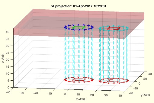 |
% VLprojection(SG,VL,ez,cent) - returns projected vertex lists on a surface/solid for given vertex list % (by Tim Lueth, VLFL-Lib, 2017-APR-01 as class: EXPERIMENTS) % % The projection surface is given as a solid. Now either by parallel % projection or central projection the resulting vertex posions on the % surface are returned. Also the distance and the index of the hit % triangles are returned. It is important to understand that the use of % EL or FL needs an additional handling, since in this case additional % points have to be created similar to SGbool. % There is also another possibility to calculate projections on % pixel/voxel accuracy using view and axes. (Status of: 2017-04-01) % % Introduced first in SolidGeometry 3.8 % % See also: VLFLpprojectPL, VLFLpprojectPLEL, crosspointVLFL, % intersectstriangle % % [VLN,DL,fi]=VLprojection([SG,VL,ez,cent]) % === INPUT PARAMETERS === % SG: SG.VL, SG.FL; solid or surface as projection plane % VL: CPL,CVL or VL as vertex list to project % ez: beam direction (cent=false) or beam origin (cent=true) % cent: central (true) or parallel projection (false); default = false; % === OUTPUT RESULTS ====== % VLN: Projected vertex list % DL: Distance list for each vertex % fi: facet index list for each point % % EXAMPLE: Try central and parallel projection % SG=SGtransP(SGbox([80,80,5]),[0 0 40]); VL=VLaddz(CPLsample(12)); % VLprojection(SG,VL,[0 0 1],false) % parallel projection % VLprojection(SG,VL,[0 0 -30],true) % central projection % % See also: VLFLpprojectPL, VLFLpprojectPLEL, crosspointVLFL, % intersectstriangle % |
exp_2017_03_30(A)- show the bounding box faces that are touched by the solid |
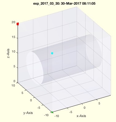 |
% exp_2017_03_30(A) - show the bounding box faces that are touched by the solid % (by Tim Lueth, VLFL-Lib, 2017-MÄR-30 as class: EXPERIMENTS) % % If STL files have been created using CATIA sometimes the Solids are % rotated slightly. This can be corrected by detecting plane surfaces and % adjust them by inverse transformation of the plane coordinate system. % Nevertheless, it is difficult to see % This fnctn is an example how to visualize the problem (Status of: % 2017-03-30) % % [XL,YL,ZL]=exp_2017_03_30(A) % === INPUT PARAMETERS === % A: Solid % === OUTPUT RESULTS ====== % XL: List of coordinate that define the X-plane % YL: List of coordinate that define the Y-plane % ZL: List of coordinate that define the Z-plane % |