SGofCPLzdelaunayGrid(CPL,z,ds,dx,dy)- returns a solid from a contour polygon list and grid resolution

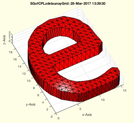% SGofCPLzdelaunayGrid(CPL,z,ds,dx,dy) - returns a solid from a contour polygon list and grid resolution % (by Tim Lüth & Christina Hein, VLFL-Lib, 2017-MÄR-27 as class: MODELING % PROCEDURES) % % The fnctn uses Delaunay-Triagulation to tesselate the base plate and % the cover plate of the part. Therefor, make sure that there are no % crossings or overlapping contours in CPL. % This fnctn will replace SGofCPLz one day since it has the same result % for the same parameter (Status of: 2017-03-29) % % See also: PLFLofCPLdelaunayGrid, CPLaddauxpoints % % SG=SGofCPLzdelaunayGrid(CPL,z,[ds,dx,dy]) % === INPUT PARAMETERS === % CPL: Contour polygon list (CPL) % z: desired height in z-coordiantes % ds: delta on the contour; default is 10000 % dx: delta grid in x; default is 10000 % dy: delta grid in y; default is dx % === OUTPUT RESULTS ====== % SG: Solid Geometry % % EXAMPLE: SGofCPLzdelaunayGrid(CPLofPL([PLcircle(20,6);NaN NaN; % flipud(PLcircle(10,4))]),10) % SGofCPLzdelaunayGrid(CPLoftext('test'),10,4,4,4) %

CPLaddauxpoints(CPL,d)- add supporting points to embedded CPL to guarantee a specified points distance

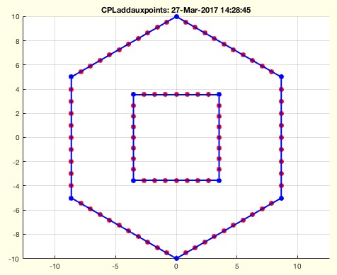% CPLaddauxpoints(CPL,d) - add supporting points to embedded CPL to guarantee a specified points distance % (by Tim Lüth & Christina Hein, VLFL-Lib, 2017-MÄR-27 as class: % AUXILIARY PROCEDURES) % % See also: SGofCPLzdelaunayGrid, PLFLofCPLdelaunayGrid, RLdelauxpoints, % GPLauxgridpointsCL, PLELaddauxpoints, GPLauxgridpointsPLEL, % RLaddauxpoints % % CPLN=CPLaddauxpoints(CPL,d) % === INPUT PARAMETERS === % CPL: Closed Polygon List % d: maximum distance between two points % === OUTPUT RESULTS ====== % CPLN: New Closed Polygon List % % EXAMPLE: % CPLaddauxpoints([PLcircle(10,6);NaN NaN; PLcircle(5,4)],1) % CPLaddauxpoints(CPLsample(12),1) %

PLFLofCPLdelaunayGrid(CPL,ds,dx,dy)- returns a point list and facet list for a grid filled contour list

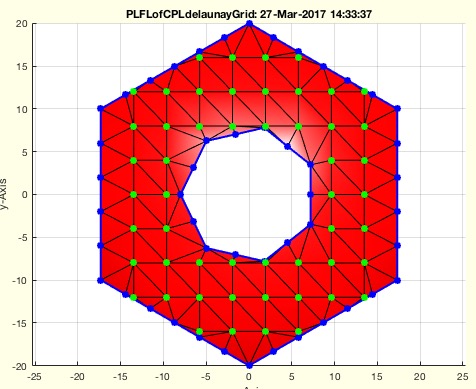% PLFLofCPLdelaunayGrid(CPL,ds,dx,dy) - returns a point list and facet list for a grid filled contour list % (by Tim Lüth & Christina Hein, VLFL-Lib, 2017-MÄR-27 as class: SURFACES) % % See also: SGofCPLzdelaunayGrid, CPLaddauxpoints % % [PL,FL,EL]=PLFLofCPLdelaunayGrid(CPL,[ds,dx,dy]) % === INPUT PARAMETERS === % CPL: Closed Polygon list % ds: delta on contour; default is 4 % dx: delta in x; default is ds % dy: delta in y; default is dx % === OUTPUT RESULTS ====== % PL: Resulting Point list % FL: Resulting Facet list % EL: Resulting Edge List % % EXAMPLE: % PLFLofCPLdelaunayGrid ([PLcircle(20,6);NaN NaN;PLcircle(8,7)]); % CPL=CPLofPL([PLcircle(20);NaN NaN; flipud(PLcircle(10))]); % PLFLofCPLdelaunayGrid(CPL,2,2) % PLFLofCPLdelaunayGrid (PLcircle(20,6)) %

VMgetSubplot- returns the current active subplot

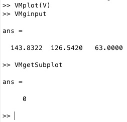% VMgetSubplot - returns the current active subplot % (by Tim Lueth, VLFL-Lib, 2017-MÄR-21 as class: USER INTERFACE) % % This fnctn returns for the VMplot figure, the number of the subplot, of % the last VMginput position was taken (Status of: 2017-03-21) % % See also: VMginput, VMplot % % subpn=VMgetSubplot % === OUTPUT RESULTS ====== % subpn: current subplot position; empty if figure is not valid %

getCurrentPoint- this function returns the currentPoint but also the axis limits

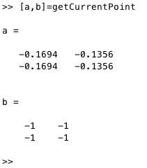% getCurrentPoint - this fnctn returns the currentPoint but also the axis limits % (by Tim Lueth, VLFL-Lib, 2017-MÄR-21 as class: USER INTERFACE) % % Sometime after ginput or after get(gca,'CurrentPoint' ) the returned % coordinates are unfortunately not inside of the active axis. This % Matlab bug is related to changing programmatically the size of the % window by a command and having at the time the windowchange allowed. % This fnctn just help to detect the problem. So it is more a debug % fnctn. (Status of: 2017-03-27) % % See also: view, get(gca, 'CurrentPoint', ) % % [p,ax]=getCurrentPoint % === OUTPUT RESULTS ====== % p: 2 point describing the view axis of the last click % ax: axis limits for each point -1 to small + 1 to big 0=inside of view %

VMginput(n,u)- returns a point position by clicking into VMplot

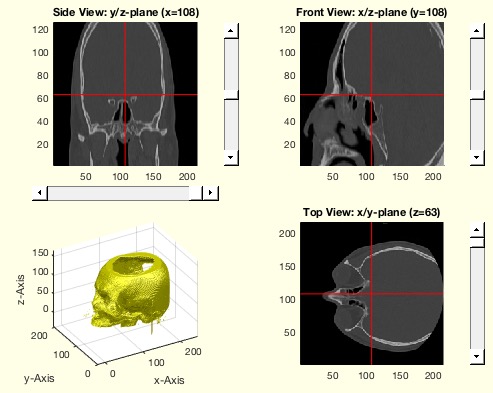% VMginput(n,u) - returns a point position by clicking into VMplot % (by Tim Lueth, VLFL-Lib, 2017-MÄR-20 as class: USER INTERFACE) % % This fnctn is based on ginput, waitforbuttonpress, % get(gca,'CurrentPoint'). % If the window is magnified, it has to be in the center of the screen % (Status of: 2017-03-21) % % See also: VMplot, VMgetSubplot % % [PL,t]=VMginput([n,u]) % === INPUT PARAMETERS === % n: number of points % u: update VMplot; default is true % === OUTPUT RESULTS ====== % PL: position % t: subplot %

SGtitle(n,w)- draws the name of the calling function as figure title

% SGtitle(n,w) - draws the name of the calling fnctn as figure title % (by Tim Lueth, Video-Lib, 2017-MÄR-19 as class: AUXILIARY PROCEDURES) % % same as title(titleofcaller,'Interpreter','none'); % (Status of: 2017-03-19) % % See also: titleofcaller % % SGtitle([n,w]) % === INPUT PARAMETERS === % n: hierarchy of calling fnctns; default is 0; % w: 'window' renames the window instead of a gca title % % EXAMPLE: % SGfigure; SGtitle % SGfigure; SGtitle(1) % SGfigure; SGtitle(-1) %

exp_2017_03_18a(A,comp)- EXPERIMENT to calculate bended surfaces

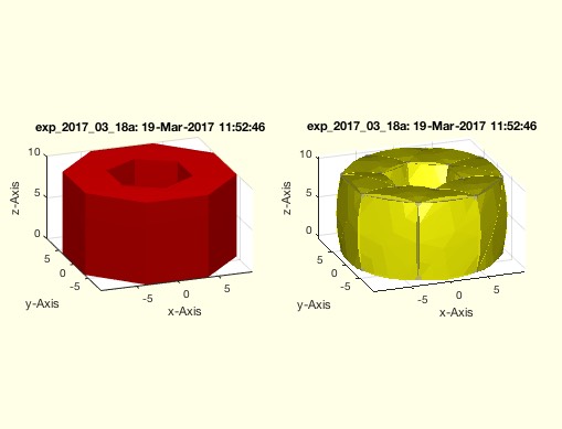% exp_2017_03_18a(A,comp) - EXPERIMENT to calculate bended surfaces % (by Tim Lueth, VLFL-Lib, 2017-MÄR-19 as class: EXPERIMENTS) % % By compressing a solid, the edges are compressed but the length of the % original edges have to be constant. The bending curve is delivered by % rofcircbend. This is done for each facet edge. In this example in % addition also the resulting solid for each face is calculated and shown. % IN THIS EXPERIMENT EACH FACET is handled separately. For complete % solids it is necessary to handle edges instead of faces. Each edge will % result in one ore more (grow) contours. (Status of: 2017-03-19) % % exp_2017_03_18a([A,comp]) % === INPUT PARAMETERS === % A: Solid Geometry % comp: compression such as 0.95 or 0.9 %

rofcircbend(s,l)- returns bending radius and angle for a compressed line

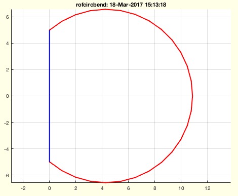% rofcircbend(s,l) - returns bending radius and angle for a compressed line % (by Tim Lueth, VLFL-Lib, 2017-MÄR-18 as class: ANALYTICAL GEOMETRY) % % the relation between a circle segment and the chord (segment crossing % line) can be solved only by a numerical search using fzero. % if s < l than the line is streched. % if s = l than the radius would be inf % if s > l there is a solution % In reality there is a minimal radius for bending because of material % stress (Status of: 2017-03-19) % % See also: lofbendinggirder, sofbendinggirder % % [r,a,PL]=rofcircbend(s,l) % === INPUT PARAMETERS === % s: original distance % l: compressed distance % === OUTPUT RESULTS ====== % r: bending radius % a: bending angle % PL: Point list describing the shape % % EXAMPLE: % rofcircbend(30,10) %

exp_2017_03_18- EXPERIMENT to solve transcendent functioon

% exp_2017_03_18 - EXPERIMENT to solve transcendent functioon % (by Tim Lueth, VLFL-Lib, 2017-MÄR-18 as class: EXPERIMENTS) % % l=2*r*sin(alpha) = 2*r*sin(b/(2*r) % alpha=b/r % (Status of: 2017-03-18) % % exp_2017_03_18 %

CVLofcontourc(C,rem)- converts the contourc format into the CVL format

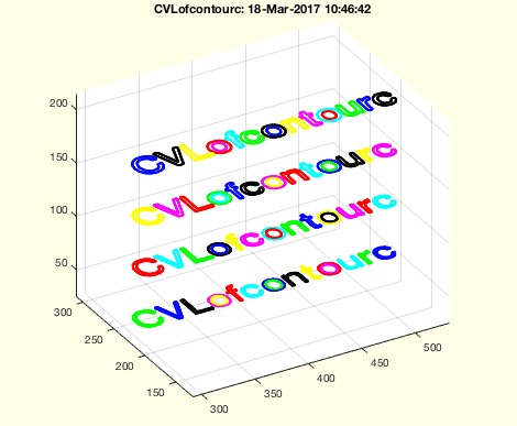% CVLofcontourc(C,rem) - converts the contourc format into the CVL format % (by Tim Lueth, VLFL-Lib, 2017-MÄR-18 as class: CLOSED POLYGON LISTS) % % Matlab's contourc fnctn is a powerful fnctn to create contours from % image bit maps similar to the marching cube fnctn in 3D. Nevertheless % the resulting point list format is outdated. This fnctn converts the % contourc format into the CVL format. The z values are the contourc % intesity(z) values. (Status of: 2017-03-18) % % See also: CPLofcontourc, contourc, CPLofimage, SGofVMdelaunay, % SGofVMmarchcube, CPLremstraight % % CVL=CVLofcontourc(C,[rem]) % === INPUT PARAMETERS === % C: result of the contourc fnctn % rem: removes straight lines if true; default is false % === OUTPUT RESULTS ====== % CVL: Closed polygon list [nx3] with the z values for the contour % % EXAMPLE: % figure; axis off; text(0.5,0.5,'This is a Test', 'FontSize',36) % I=getframe(gcf); % CVLofcontourc(contourc(1/3*sum(flipud(I.cdata),3),4)) %

CPLcontourc(Inputparameter)- returns the CPL of matlab's contourc command

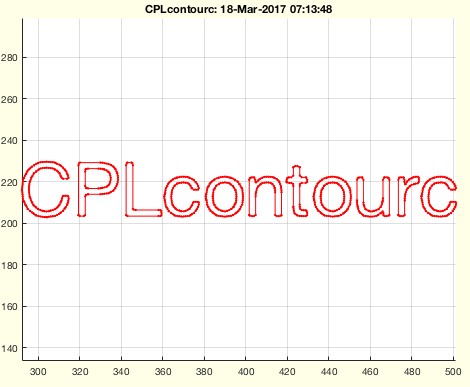% CPLcontourc(Inputparameter) - returns the CPL of matlab's contourc command % (by Tim Lueth, VLFL-Lib, 2017-MÄR-18 as class: CLOSED POLYGON LISTS) % % This fnctn simply calls contourc and converts the output matrix into % CPL format. % For the properties of the contour matrix result read the help for % ContourMatrix % ATTENTION: The original ContourMatrix supports open and closed PL! % ATTENTION: The original ContourMatrix has many points on a staight line! % Automatically converts the type into the requested double format. % (Status of: 2017-05-24) % % See also: PLofimcontourc, CVLofcontourc, CPLofcontourc, contourc, % ContourMatrix, % https://de.mathworks.com/help/matlab/ref/contour-properties.html % % CPL=CPLcontourc([Inputparameter]) % === INPUT PARAMETERS === % Inputparameter: exactly the parameter same as contourc % === OUTPUT RESULTS ====== % CPL: Closed polygon list % % EXAMPLE: % figure; axis off; text(0.5,0.5,'This is a Test', 'FontSize',36) % I=getframe(gcf); I=flipud(I.cdata(:,:,1)); % CPLcontourc(I,1); %

smbCreateSpring(M1,M2,SGName,len,sprg,damp)- smb creates a spring damper link between two point masses

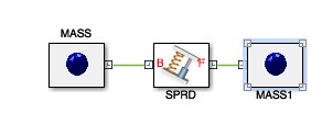% smbCreateSpring(M1,M2,SGName,len,sprg,damp) - smb creates a spring damper link between two point masses % (by Tim Lueth, SimMechanics, 2017-MÄR-17) % % M1 and M2 are connected using LConn1 (Status of: 2017-03-17) % % See also: smbNewSystem, smbCreateSGMass % % h=smbCreateSpring(M1,M2,[SGName,len,sprg,damp]) % === INPUT PARAMETERS === % M1: Mass 1 % M2: Mass 2 % SGName: optional name; default is 'SPRD; % len: len in mm % sprg: spring constant in N/m % damp: Damping in N/(m/s) % === OUTPUT RESULTS ====== % h: spring-damper block % % EXAMPLE: % smbNewSystem ('smb_exp_2017_03_17b',[0 0 -9.81]); % M1=smbCreateSGMass; % M2=smbCreateSGMass; % smbCreateSpring(M1,M2); % smbAddLine( 'WORLD/RConn1', [M1 '/LConn1']); %

smbCreateSGMass (SG,SGName,SGcol)- smbcreates a double mass model with random inertia and point mass

% smbCreateSGMass (SG,SGName,SGcol) - smbcreates a double mass model with random inertia and point mass % (by Tim Lueth, SimMechanics, 2017-MÄR-17 as class: MODELING PROCEDURES) % % Since smb start the movement in the origin, it is very easy to create % singularity condition without intention. Therefor, this fnctn links a % point mass with a random inertia deviation to create objects that can % be connected by springs (Status of: 2017-03-17) % % See also: smbNewSystem, smbCreateSpring % % smbCreateSGMass([SG,SGName,SGcol]) % === INPUT PARAMETERS === % SG: Solid Geometry; default is a sphere with radius 1 % SGName: Optional Name; default is 'MASS' % SGcol: Optional Color % % EXAMPLE: % smbNewSystem ('smb_exp_2017_03_17b',[0 0 -9.81]); % M1=smbCreateSGMass; % M2=smbCreateSGMass; % smbCreateSpring(M1,M2); % smbAddLine( 'WORLD/RConn1', [M1 '/LConn1']); %

exp_2017_03_17- EXPERIMENT to show falling and oscillation of a mass point

% exp_2017_03_17 - EXPERIMENT to show falling and oscillation of a mass point % (by Tim Lueth, VLFL-Lib, 2017-MÄR-17 as class: EXPERIMENTS) % % This is the basic experiment for mass spring damper systems, starting % the simulation all in the origin (Status of: 2017-03-17) % % exp_2017_03_17 %

SGmodelMass(R)- creates a mass point including 2 frames

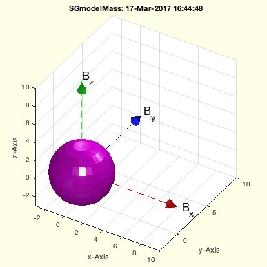% SGmodelMass(R) - creates a mass point including 2 frames % (by Tim Lueth, VLFL-Lib, 2017-MÄR-17 as class: SIMMECHANICS INTERFACE) % % See also: SGmodelLink, SGmodelJoint, SGmodelNode, SGmodelLink3, % SGmodelKeyhole, SGmodelLink1, SGmodelLink2 % % SG=SGmodelMass([R]) % === INPUT PARAMETERS === % R: Radius % === OUTPUT RESULTS ====== % SG: Solid geometry % % EXAMPLE: % SGmodelMass(8) %

CPLoftext(str,siz,FW,FN)- returns a CPL of one or more textlines separated by \n

% CPLoftext(str,siz,FW,FN) - returns a CPL of one or more textlines separated by \n % (by Tim Lueth, VLFL-Lib, 2017-MÄR-17 as class: CLOSED POLYGON LISTS) % % This fnctn takes seconds to process. % 10 point ~ 7 mm "g' to 'X' is about 10mm, a line is about 14 mm (Status % of: 2017-03-17) % % See also: CPLofimage, CPLofcontourc, textHorizontalBlockAlign % % CPL=CPLoftext(str,[siz,FW,FN]) % === INPUT PARAMETERS === % str: one or more textlines separated by \n % siz: size in pt % FW: FontWidth; see text; default is 'normal' % FN: FontName; see text; default is 'Helevetica' % === OUTPUT RESULTS ====== % CPL: Closed Polygon Line % % EXAMPLE: % tic; CPLoftext('test',0.2); toc; % tic; CPLoftext('test',70); toc; % SGofCPLz(CPLoftext('test'),5); view(-30,30); % CPLoftext('The quick brown fox jumps\n over the lazy % dog',10,'bold','Cambria') %

FLofCPL(CPL)- misleading function - use PLFLofCPLdelaunay, PLFLofCPLpoly instead

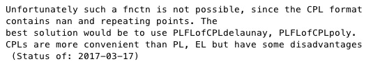% FLofCPL(CPL) - misleading fnctn - use PLFLofCPLdelaunay, PLFLofCPLpoly instead % (by Tim Lueth, Video-Lib, 2017-MÄR-17 as class: CLOSED POLYGON LISTS) % % Unfortunately such a fnctn is not possible, since the CPL format % contains nan and repeating points. The best solution would be to use % PLFLofCPLdelaunay or PLFLofCPLpoly. % CPLs are more convenient than PL, EL but have some disadvantages % (Status of: 2017-03-17) % % See also: PLFLofCPLpoly, PLFLofCPLdelaunay, PLELofCPL, FLofPLEL % % FL=FLofCPL(CPL) % === INPUT PARAMETERS === % CPL: Closed Polygon List % === OUTPUT RESULTS ====== % FL: Facet List % % EXAMPLE: Try instead % PLFLofCPLdelaunay(CPL) % %

CPLofcontourc(C,rem)- converts the contourc format into the CPL format

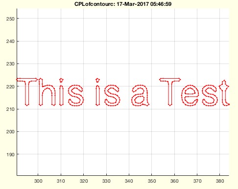% CPLofcontourc(C,rem) - converts the contourc format into the CPL format % (by Tim Lueth, VLFL-Lib, 2017-MÄR-17 as class: CLOSED POLYGON LISTS) % % Matlab's contourc fnctn is a powerful fnctn to create contours from % image bit maps similar to the marching cube fnctn in 3D. Nevertheless % the resulting point list format is outdated. This fnctn converts the % contourc format into the CPL format. (Status of: 2017-03-18) % % See also: CVLofcontourc, contourc, CPLofimage, SGofVMdelaunay, % SGofVMmarchcube, CPLremstraight % % CPL=CPLofcontourc(C,[rem]) % === INPUT PARAMETERS === % C: result of the contourc fnctn % rem: removes straight lines if true; default is true % === OUTPUT RESULTS ====== % CPL: Closed polygon list % % EXAMPLE: % figure; axis off; text(0.5,0.5,'This is a Test', 'FontSize',36) % I=getframe(gcf); I=flipud(I.cdata(:,:,1)); C=contourc(double(I),1); % CPLofcontourc(C) %

VLofimage(I,pixsize,h,nf)- converts an image into a contour or a solid

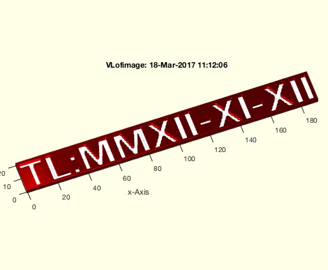% VLofimage(I,pixsize,h,nf) - converts an image into a contour or a solid % (by Tim Lueth, VLFL-Lib, 2017-MÄR-16 as class: TEXT PROCEDURES) % % Rewritten based on the contour fnctn. Quite useful procedure to % generate contours from images or string comments in combination with % imageoftext. If parameter h>0, the fnctn returns a solid. % There is an earlier version, now called VLofimage_2012b. (Status of: % 2017-03-18) % % See also: CPLtextimage, VLFLtextimage, imageoftext % % [VL,EL,FL,CPL]=VLofimage(I,[pixsize,h,nf]) % === INPUT PARAMETERS === % I: image array % pixsize: size of a pixel % h: desired heigth; default is 0 (Contour) % nf: frame in pixels; if nf>0 the image is impressed; default is 0 % === OUTPUT RESULTS ====== % VL: Vertex list (nx2) for h=0; (nx3) for h>0; % EL: Edge list % FL: Facet list % CPL: Closed Polygon list based on contour % % EXAMPLE: Generate a contour for the string 'Test': % I=imageoftext('TL:MMXII-XI-XII',36); % [VL,EL,FL]=VLofimage(I,.7); VLELplot(VLaddz(VL),EL,'r-') % [VL,EL,FL]=VLofimage(I,.7,3); close all, VLFLplot(VL,FL), %

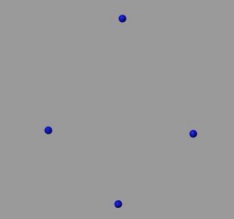
CPLofimage(I,n,f)- returns a point list related to matlab;s contour function

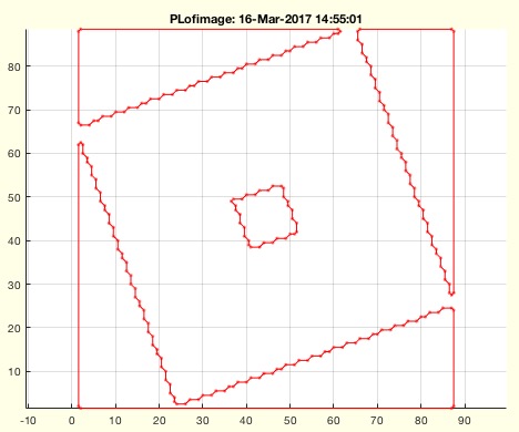% CPLofimage(I,n,f) - returns a point list related to matlab;s contour fnctn % (by Tim Lueth, VLFL-Lib, 2017-MÄR-16 as class: CLOSED POLYGON LISTS) % % based on matlab's contour to accelerate the fnctn VLofimage. If image I % is a struct, I is converted into a gray scale image by: % I=1/s(3)*sum(I.cdata,3) % (Status of: 2017-03-17) % % See also: CPLremstraight, VLofimage % % CPL=CPLofimage(I,[n,f]) % === INPUT PARAMETERS === % I: image % n: number of contours % f: if true create a zero frame around; default is false % === OUTPUT RESULTS ====== % CPL: Closed Polygon List % % EXAMPLE: % figure; axis off; text(0.5,0.5,'This is a Test', 'FontSize',16); % I=getframe(gcf) % CPLofimage(I) % CPLofimage(I.cdata(:,:,1)<240) % I.cdata=squeeze(I.cdata(:,:,1)); CPLofimage(I) %

CPLsortinout(CPL,in1st)- returns a inside outside sorted CPL

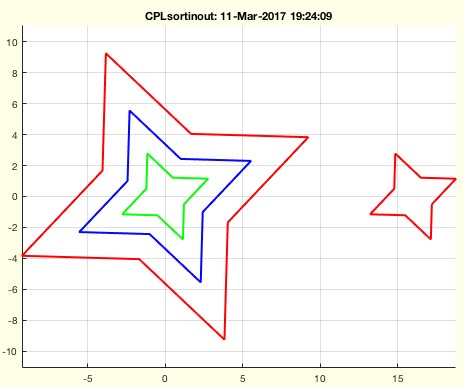% CPLsortinout(CPL,in1st) - returns a inside outside sorted CPL % (by Tim Lueth, VLFL-Lib, 2017-MÄR-11 as class: CLOSED POLYGON LISTS) % % For laser cutting, the insider first order is required. For automatic % detection of corresponding vessels, outside first is important. % Corresponance matrix: % (i,j)==+1 i is inside j, -1== i is outside j, NaN==crossing % (Status of: 2017-06-04) % % See also: connectofmat, selectNaN, separateNaN, CPLisccwinout, % svgpolylineofCPL, CPLwriteSVG % % [cind,CC,NCPL,pi]=CPLsortinout([CPL,in1st]) % === INPUT PARAMETERS === % CPL: Original CPL % in1st: true==inside first; false=outside first; default is true % === OUTPUT RESULTS ====== % cind: level index related to separatedNaN (CPL) % CC: Corresponance matrix % NCPL: New contour list sorted by enclosure order % pi: parent index list % % EXAMPLE: % CPLsortinout(selectNaN(CPLsample(14),[1,2,3,6])) % CPLsortinout(selectNaN(CPLsample(14),[1,2,3,6]),false) % [~,CC]=CPLsortinout(CPLsample(14)); c=connectofmat(CC) %

selectNaN(CPL,ci)- connects subsets of closed polygons lines (2D/3D) wrt an index list

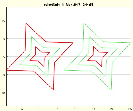% selectNaN(CPL,ci) - connects subsets of closed polygons lines (2D/3D) wrt an index list % (by Tim Lueth, VLFL-Lib, 2017-MÄR-11 as class: CLOSED POLYGON LISTS) % % See also: separateNaN, replaceNaN, cellofNaN % % CPLN=selectNaN(CPL,ci) % === INPUT PARAMETERS === % CPL: CPL / CVL % ci: index list [ % === OUTPUT RESULTS ====== % CPLN: Subset of CPL or new ordered CPL % % EXAMPLE: Select 3 CPL of CPLsample(14) % selectNaN(VLaddz(CPLsample(14),pi),[1,3,6]) %

movepathtotop (pstr)- moves a search path from its current position to the beginning of the search path

% movepathtotop (pstr) - moves a search path from its current position to the beginning of the search path % (by Forian Schleich & Tim Lueth, VLFL-Lib, 2017-MÄR-11 as class: % AUXILIARY PROCEDURES) % % Some libraries such as VLFL-Lib or SG-Lib overload unfortunately % existing fnctns such as roundN. Nevertheless, by using the fnctn the % relevant library can be moved to the top. (Status of: 2017-03-11) % % See also: VLFLlicense % % movepathtotop([pstr]) % === INPUT PARAMETERS === % pstr: fullpath of a search directory; default is rec of %

RRcputime(RRtictime)- returns realtime difference and cputime difference since first call

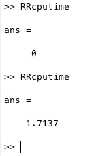% RRcputime(RRtictime) - returns realtime difference and cputime difference since first call % (by Christian Dietz, VLFL-Lib, 2017-MÄR-09 as class: AUXILIARY % PROCEDURES) % % If Matlab works with 100% CPU time, tic time and CPU time are % identical. Nevertheless, is makes sense also to check the Realtime in % realtime systems :-) (Status of: 2017-03-09) % % See also: RRrun % % [t,tc]=RRcputime([RRtictime]) % === INPUT PARAMETERS === % RRtictime: only used for reset by tic % === OUTPUT RESULTS ====== % t: time difference since first call % tc: CPUtime difference since first call %

plotannotation(str,)- plots a annotation box into the right upper corner of a plot

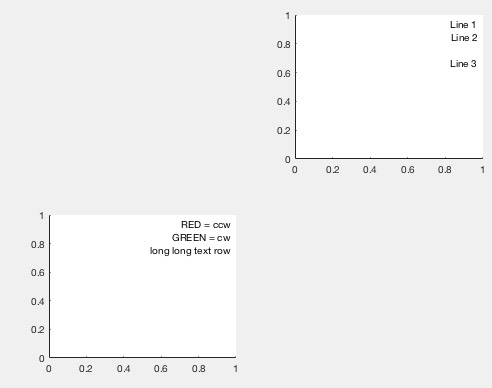% plotannotation(str,) - plots a annotation box into the right upper corner of a plot % (by Tim Lueth, VLFL-Lib, 2017-MÄR-09 as class: USER INTERFACE) % % the annotation box is able to adjust the size but this fnctn is related % to the "left" "HorizontalAlignment". Therefor it is necessary to % calculate a little to bring an automatical size adjusted box into the % right corner of a subplot (Status of: 2017-03-09) % % See also: annotation, titleofcaller % % t=plotannotation(str,[]) % === INPUT PARAMETERS === % str: string or cell with separated strings % === OUTPUT RESULTS ====== % t: handle to annotation box % % EXAMPLE: % subplot(2,2,3); % t=plotannotation({'RED = ccw','GREEN = cw','long long text % row'},'linestyle','none'); % subplot(2,2,2); % t=plotannotation('Line 1\n Line 2\n\nLine 3','linestyle','none'); % %