New in SG-Lib 2.8
depfunTL(fname,par)- returns all dependency files of a function that are not part of a toolbox |
 |
% depfunTL(fname,par) - returns all dependency files of a fnctn that are not part of a toolbox % (by Tim Lueth, VLFL-Lib, 2016-JUN-05 as class: AUXILIARY PROCEDURES) % % This fnctn is using instad of depfun (2014b) now comptabile to 2015a % the fnctn matlab.codetools.requiredFilesAndProducts. It works similar % to depfun ('fnctnname'), which without '-toponly' seems to be instable % in 2012b % depfunTL shows all procedures that are used in a procedure % depuseTL shows all procedures that uses a named procedure % % Will be replaced by % a=matlab.codetools.requiredFilesAndProducts('exp_2015_09_30') % % (Status of: 2017-01-03) % % See also: publishTL, pcodeTL, depuseTL, depuseString % % [PL,ML]=depfunTL(fname,[par]) % === INPUT PARAMETERS === % fname: fnctn name % par: parameter such as '-toponly' % === OUTPUT RESULTS ====== % PL: List of private fnctns % ML: List of matlab fnctns % % EXAMPLE: Depency files of FTelement.m % depfunTL ('FTelement') % % |
exp_2016_02_20- EXPERIMENT to create graphs and FEM networks |
 |
%% HAND-OUT: EXP_2016_02_20 EXPERIMENT TO CREATE GRAPHS AND FEM NETWORKS % * (by Tim Lueth, VLFL-Lib, 2016-FEB-20 as class: EXPERIMENTS) % * *Please feel free to read it - and put it back* % * *If somebody is interested in this document, please ask Tim Lueth for an additional copy* %% % exp_2016_02_20 - EXPERIMENT to create graphs and FEM networks % (by Tim Lueth, VLFL-Lib, 2016-FEB-20 as class: EXPERIMENTS) % % This experiment is initiated by reading the book of Frank-Thomas % Mellert (1980) "Rechnergestützter Entwurf elektrischer Schaltungen" % explaining the background of electrical network analysis programs known % as SPICE. (The book was a gift of Wolfgang Hilberg to Tim Lueth, Nov % 1986. It was an addition to the introduction of the "Modified Node % Analyses" explained by Martin Bossert to Tim Lueth in Nov. 1985.) Part % of the second chapter is a short explanation how to solve linear % equation systems and partial differential equation systems using % numerical mathematics. % Tim Lueth is interested to implement the methods in MATLAB since those % equation systems are the basics of statics (structural analysis), % elastostatics of rigid bodies and textiles as well as of electrical % networks. % % (Status of: 2016-02-21) % % LITERATURE: % - Frank-Thomas Mellert (1981): Rechnergestützter Entwurf elektrischer % Schaltungen, Oldenbourg, München % % exp_2016_02_20 % |
centerVL(VL)- returns the center and distance indices of a vertex list |
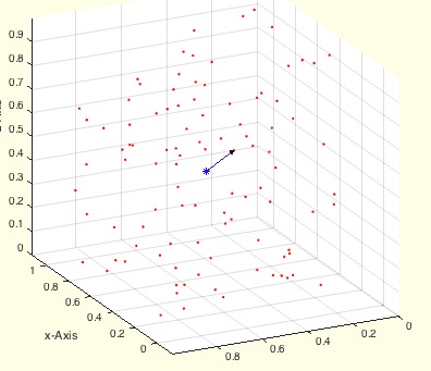 |
% centerVL(VL) - returns the center and distance indices of a vertex list % (by Tim Lueth, VLFL-Lib, 2016-FEB-14 as class: ANALYTICAL GEOMETRY) % % Auxiliary fnctn to find nearest points to a cloud center (Status of: % 2017-02-01) % % See also: center3P, center4P, centerPL % % [c,ci,d,n]=centerVL(VL) % === INPUT PARAMETERS === % VL: Vertex list (nx3) % === OUTPUT RESULTS ====== % c: center % ci: index list of nearest vertices % d: distance vector to center (nx3) % n: distance norm to center (nx1) % % EXAMPLE: Show the center of a random list % centerVL (rand(100,3)) % |
exp_2016_02_13- EXPERIMENT to create graphs and FEM networks |
 |
%% HAND-OUT: EXP_2016_02_13 EXPERIMENT TO CREATE GRAPHS AND FEM NETWORKS % * (by Tim Lueth, VLFL-Lib, 2016-FEB-13 as class: EXPERIMENTS) % * *Please feel free to read it - and put it back* % * *If somebody is interested in this document, please ask Tim Lueth for an additional copy* %% % exp_2016_02_13 - EXPERIMENT to create graphs and FEM networks % (by Tim Lueth, VLFL-Lib, 2016-FEB-13 as class: EXPERIMENTS) % % This experiment is initiated by reading the book of Frank-Thomas % Mellert (1980) "Rechnergestützter Entwurf elektrischer Schaltungen" % explaining the background of electrical network analysis programs known % as SPICE. (The book was a gift of Wolfgang Hilberg to Tim Lueth, Nov % 1986. It was an addition to the introduction of the "Modified Node % Analyses" explained by Martin Bossert to Tim Lueth in Nov. 1985.) Part % of the second chapter is a short explanation how to solve linear % equation systems and partial differential equation systems using % numerical mathematics. % Tim Lueth is interested to implement the methods in MATLAB since those % equation systems are the basics of statics (structural analysis), % elastostatics of rigid bodies and textiles as well as of electrical % networks. % % (Status of: 2016-02-15) % % [VL,FL,BL,A,VT]=exp_2016_02_13 % === OUTPUT RESULTS ====== % VL: Vertex list % FL: Facet list % BL: Bow list (arbitrarily directed edges) % A: Bow-Edge-Incidence-Matrix % VT: Vertex tree (n x [end vi,bow, start vi]) % |
VLFLplotlightoff- switches the camlights on or off |
 |
% VLFLplotlightoff - switches the camlights on or off % (by Tim Lueth, VLFL-Lib, 2016-JAN-10 as class: VISUALIZATION) % % VLFLplotlightoff % |
implot(I,newx,z)- plots an image as scaled texture |
 |
% implot(I,newx,z) - plots an image as scaled texture % (by Tim Lueth, VLFL-Lib, 2016-JAN-10 as class: VISUALIZATION) % % h=implot(I,newx,z) % === INPUT PARAMETERS === % I: imagex % newx: length of the xaxis % z: % === OUTPUT RESULTS ====== % h: handle % |
exp_2016_01_10;- EXPERIMENT |
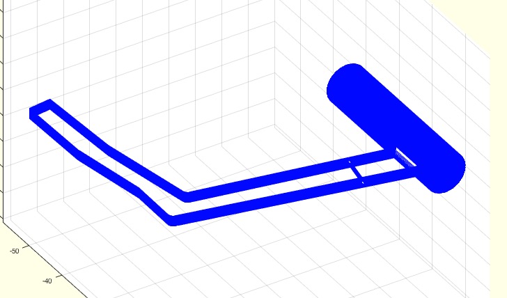 |
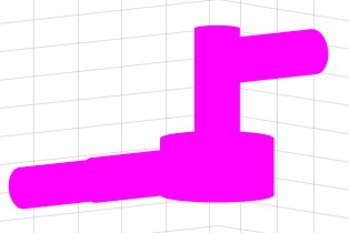
%% PUBLISHABLE EXP_2016_01_10; EXPERIMENT % (by Tim Lueth, VLFL-Lib, 2016-JAN-10 as class: EXPERIMENTS) %% % exp_2016_01_10; - EXPERIMENT % (by Tim Lueth, VLFL-Lib, 2016-JAN-10 as class: EXPERIMENTS) % % Tim Lueth got 3 bended bars from Marcus Rompf on 2015-01-09 of an % accordion bass mechanic. TL's goal (Status of: 2016-01-10) % % SG=exp_2016_01_10; % === OUTPUT RESULTS ====== % SG: Solid Geometry % |
SGvolume(SG,sz)- returns the estimated volume of a solid |
 |
% SGvolume(SG,sz) - returns the estimated volume of a solid % (by Tim Lueth, VLFL-Lib, 2016-JAN-10 as class: ANALYTICAL GEOMETRY) % % In contrast to SGweight, this procedure slices the solid. It uses % procedure CPLofSGslice2 (Status of: 2016-01-10) % % See also: SGweight, SGvolume, CPLofSGslice2, SGseparate, CPLofSGslice % % [VSUM,A]=SGvolume(SG,[sz]) % === INPUT PARAMETERS === % SG: Solid Geoemtry % sz: step size in z; default is 1 % === OUTPUT RESULTS ====== % VSUM: Volume in cm^3 % A: Area of the individual slices % |
CPLarea(CPL,sep)- returns the area of the surfaces (VL/PL) |
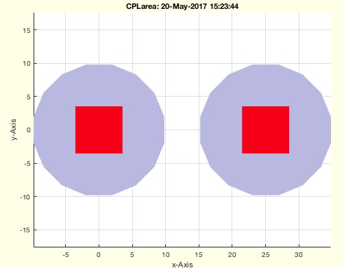 |
% CPLarea(CPL,sep) - returns the area of the surfaces (VL/PL) % (by Tim Lueth, VLFL-Lib, 2016-JAN-10 as class: SURFACES) % % With respect to Heron: A=sqrt(s(s-a)(s-b)(S-c)); s=0.5*(a+b+c). % (Status of: 2017-05-20) % % See also: SGarea, VLFLarea % % [ASUM,A]=CPLarea(CPL,[sep]) % === INPUT PARAMETERS === % CPL: Closed Polygon List % sep: true=calculate each contour separately; default is false % === OUTPUT RESULTS ====== % ASUM: Area of the surfaces % A: Area list for facet list % % EXAMPLE: Try: % CPLarea(CPLsample(12)) % CPLarea(CPLsample(12),true) % |
SGarea(SG)- returns the area of the surfaces (VL/PL) |
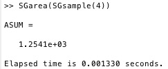 |
% SGarea(SG) - returns the area of the surfaces (VL/PL) % (by Tim Lueth, VLFL-Lib, 2016-JAN-10 as class: SURFACES) % % With respect to Heron: A=sqrt(s(s-a)(s-b)(S-c)); s=0.5*(a+b+c). % (Status of: 2016-01-10) % % See also: SGarea, VLFLarea, CPLarea % % [ASUM,A]=SGarea(SG) % === INPUT PARAMETERS === % SG: Solid Geoemtry % === OUTPUT RESULTS ====== % ASUM: Area of the surfaces % A: Area list for facet list % % EXAMPLE: Try: % SGarea(SGbox([30,20,10]) % |
VLFLarea(VL,FL)- returns the area of the surfaces (VL/PL) |
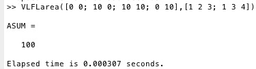 |
% VLFLarea(VL,FL) - returns the area of the surfaces (VL/PL) % (by Tim Lueth, VLFL-Lib, 2016-JAN-10 as class: SURFACES) % % With respect to Heron: A=sqrt(s(s-a)(s-b)(S-c)); s=0.5*(a+b+c). % This procedure support point lists (2D) or vertex lists (3D) % (Status of: 2016-01-10) % % See also: SGarea, VLFLarea, CPLarea % % [ASUM,A]=VLFLarea(VL,FL) % === INPUT PARAMETERS === % VL: Vertex list (nx3) or Point List (nx2) % FL: Facet list % === OUTPUT RESULTS ====== % ASUM: Area of the surfaces % A: Area list for facet list % % EXAMPLE: Try: % VLFLarea([0 0; 10 0; 10 10; 0 10],[1 2 3; 1 3 4]) % |
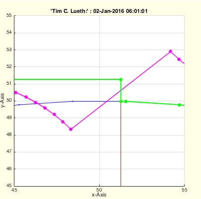
synth4Bar3Pose(C1,D1,C2,D2,C3,D3,d)- returns 4 points for a 4 Bar linkage |
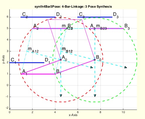 |
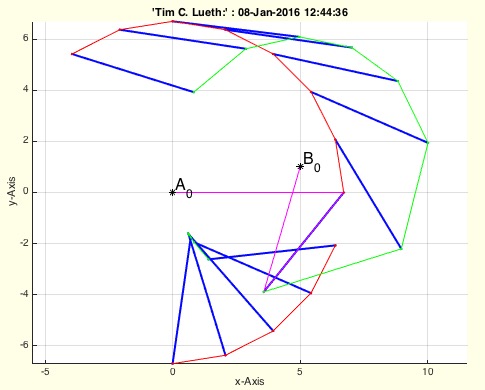
% synth4Bar3Pose(C1,D1,C2,D2,C3,D3,d) - returns 4 points for a 4 Bar % linkage % (by Tim Lueth, VLFL-Lib, 2016-JAN-08 as class: KINEMATICS AND FRAMES) % % 3 Pose synthesis for a 4 Bar Linkage based on two specified poses: By % describing 3 coupler poses by 2 points (C1_D1, C2_D2, C3_D3) each. % (Status of: 2016-01-08) % % See also: synth4Bar2Pose, plot4Bar, calc4BarAngle, cross2circ, % synth4Bar3Pose, % % LITERATURE: % - Kerle, H., Pittschellis, R. Corves, B. (2007): Einführung in die % Getriebelehre, B.G. Teubner Verlag, 3. Auflage % % [A0,B0,A1,B1]=synth4Bar3Pose(C1,D1,C2,D2,C3,D3,[d]) % === INPUT PARAMETERS === % C1: Coupler point C Pose 1 % D1: Coupler point D Pose 1 % C2: Coupler point C Pose 2 % D2: Coupler point D Pose 2 % C3: Coupler point C Pose 3 % D3: Coupler point D Pose 3 % d: distance from C1/C2/C3 to A1/A2/A3; default [1 -1] % === OUTPUT RESULTS ====== % A0: Base link A % B0: Base link B % A1: End link A % B1: End link B % % EXAMPLE: Try % synth4Bar3Pose([0 2],[3 2],[1 6],[5 6],[6 5],[8 5]) % |
plot4Bar(A0,B0,A1,B1,wl,cc)- plots a 4-Bar-linkage |
 |
% plot4Bar(A0,B0,A1,B1,wl,cc) - plots a 4-Bar-linkage % (by Tim Lueth, VLFL-Lib, 2016-JAN-08 as class: KINEMATICS AND FRAMES) % % simple procedure to animate the movement of a 4-Bar-linkage. Uses % calc4BarAngle for movement calcualtion (Status of: 2016-01-08) % % See also: plot4Bar, calc4BarAngle, synth4Bar2Pose, cross2circ % % plot4Bar(A0,B0,A1,B1,[wl,cc]) % === INPUT PARAMETERS === % A0: Base point of link A % B0: Base point of link B % A1: End point of link A % B1: End point of link B % wl: list of angles; default is [0..2pi] % cc: color of the coupler; default is '' % % EXAMPLE: Try % SGfigure; plot4Bar([0 0],[5 1],[6 3],[10 0],'','b-') % |
calc4BarAngle(A0,B0,A1,lb,lc)- returns 4-Bar-Linkage points for link B |
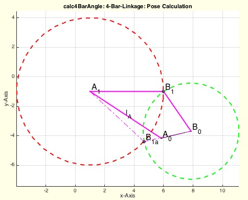 |
% calc4BarAngle(A0,B0,A1,lb,lc) - returns 4-Bar-Linkage points for link B % (by Tim Lueth, VLFL-Lib, 2016-JAN-08 as class: KINEMATICS AND FRAMES) % % calculation of the end point(s) of link B of a 4-Bar-linkage for a % given position. (Status of: 2016-01-08) % % See also: calc4BarAngle, synth4Bar2Pose, cross2circ % % [B1,B1a,x,y,e,o]=calc4BarAngle(A0,B0,A1,lb,lc) % === INPUT PARAMETERS === % A0: Base point of link A % B0: Base point of link B % A1: Position of point A1 % lb: length of link B % lc: length of coupler (A1B1) % === OUTPUT RESULTS ====== % B1: Right hand solution for positive x % B1a: Left hand solution for positive x % x: straight distance from A1B0 % y: orthogonal distance from A1B0 % e: unit vector A1B0 % o: orthogonal vector A1B0 % % EXAMPLE: try % calc4BarAngle ([0 0],[4 0],[-1 5],2,6) % |
cross2circ(A0,B0,ra,rb);- returns the crossing points of two circles |
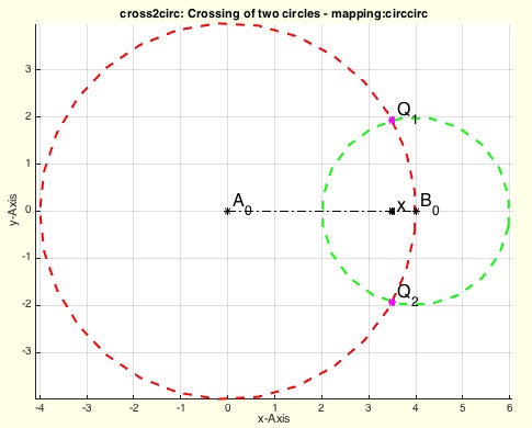 |
% cross2circ(A0,B0,ra,rb); - returns the crossing points of two circles % (by Tim Lueth, VLFL-Lib, 2016-JAN-08 as class: ANALYTICAL GEOMETRY) % % Similar to circcirc (mapping toolbox) but without using a toolbox plus % drawing the result. Only real solutions are return; else NaN NaN % (Status of: 2016-01-08) % % See also: circcirc % % [Q1,Q2,x,y,e,o]=cross2circ(A0,B0,ra,rb); % === INPUT PARAMETERS === % A0: Center of circle A % B0: Center of circle B % ra: Radius of circle A % rb: Radius of circle B % === OUTPUT RESULTS ====== % Q1: Solution right hand to A0B0 for positive x % Q2: Solution left hand to A0B0 for positive x % x: distance from A0 to B0 % y: orthogonal from A0+e*x % e: unit direction vector % o: unit orthogonal vector % % EXAMPLE: try % cross2circ([0 0],[4 0],4,2) % 2 Solutions % cross2circ([0 0],[4 0],2,2) % 1 Solution % cross2circ([0 0],[4 0],2,2) % No Solution % cross2circ([0 0],[4 0],1,6) % No Solution % |
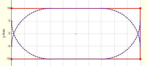
synth4Bar2Pose(C1,D1,C2,D2,d,la,lb)- returns 4 points for a 4 Bar linkage |
 |
% synth4Bar2Pose(C1,D1,C2,D2,d,la,lb) - returns 4 points for a 4 Bar % linkage % (by Tim Lueth, VLFL-Lib, 2016-JAN-07 as class: KINEMATICS AND FRAMES) % % 2 Pose synthesis for a 4 Bar Linkage based on two specified poses: By % describing 2 coupler poses by 2 points (C1-D1 and C2-D2) each, the two % lines are constructed where the base frames A0 and B0 must be located. % The coupler may have a fixed location relative to the links A0-A1 and % B0-B1. Also it is possible to give an exact distance for A0 and B0 from % the middle points mA and mB. (Status of: 2016-01-08) % % See also: synth4Bar2Pose, plot4Bar, calc4BarAngle, cross2circ % % LITERATURE: % Kerle, H., Pittschellis, R. Corves, B. (2007): Einführung in die % Getriebelehre, B.G. Teubner Verlag, 3. Auflage % % [A0,B0,A1,B1,P12]=synth4Bar2Pose(C1,D1,C2,D2,[d,la,lb]) % === INPUT PARAMETERS === % C1: Coupler point C Pose 1 % D1: Coupler point D Pose 1 % C2: Coupler point C Pose 2 % D2: Coupler point D Pose 2 % d: distance from C1/C2/ to A1/A2 % la: length from mA to A0 % lb: length from mB to B0 % === OUTPUT RESULTS ====== % A0: Base link A % B0: Base link B % A1: End link A % B1: End link B % P12: Pole (A0=B0) % % EXAMPLE: Try % synth4Bar2Pose([0 0],[5 0],[6 3],[10 0]) % synth4Bar2Pose([0 2],[5 2],[0 5],[5 5]) % synth4Bar2Pose([0 0],[5 0],[6 3],[10 0],[0 -1],0,0) % % |
CPLofSGslice2(SG,z)- return slices of a separated SG |
 |
% CPLofSGslice2(SG,z) - return slices of a separated SG % (by Tim Lueth, VLFL-Lib, 2016-JAN-07 as class: SLICES) % % Same as SGslice, but does support separated objects. It also has % includes code that corrects problems by vertices near the slicing % plane. (Status of: 2016-01-07) % % See also: CPLofSGslice, CPLofSGslice2 % % CPL=CPLofSGslice2(SG,z) % === INPUT PARAMETERS === % SG: Solid geometry; incl. separated objects % z: z-plane to slice % === OUTPUT RESULTS ====== % CPL: CPL of the sliced plane % |
TofDPhi(D,Phi)- returns a 3x3 HT matrix for 2D link |
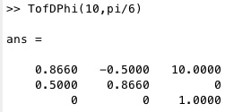 |
% TofDPhi(D,Phi) - returns a 3x3 HT matrix for 2D link % (by Tim Lueth, HT-Lib, 2016-JAN-07 as class: KINEMATICS AND FRAMES) % % Similar to VLtransR, VLtransP, VLtransT (Status of: 2017-01-29) % % See also: TofR, TofVL, TPL, TofDPhiH, T3ofT2, T3P, T2P, TofP, TofPez, % TofPEul % % T=TofDPhi(D,Phi) % === INPUT PARAMETERS === % D: Distance in X % Phi: rotation around Z % === OUTPUT RESULTS ====== % T: 3x3 HT matrix (2D) % |
T3ofT2(T)- converts a 3x3 HT-Matrix into a 4x4 HT-Matrix |
 |
% T3ofT2(T) - converts a 3x3 HT-Matrix into a 4x4 HT-Matrix % (by Tim Lueth, HT-Lib, 2016-JAN-06 as class: KINEMATICS AND FRAMES) % % helpful for planar mechanism desgin (Status of: 2017-01-21) % % See also: TofR, TofVL, TPL, TofDPhiH, T3P, T2P % % T=T3ofT2(T) % === INPUT PARAMETERS === % T: 3x3 HT Matrix % === OUTPUT RESULTS ====== % T: 4x4 HT Matrix % |
TofR(R,t)- returns a HT matrix for an R matrix |
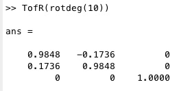 |
% TofR(R,t) - returns a HT matrix for an R matrix % (by Tim Lueth, HT-Lib, 2016-JAN-06 as class: KINEMATICS AND FRAMES) % % Supports 2x2 and 3x3 rotation matrices. (Status of: 2017-01-29) % % See also: TofR, TofVL, TPL, TofDPhiH, T3ofT2, T3P, T2P, TofP, TofPez, % TofPEul % % T=TofR(R,[t]) % === INPUT PARAMETERS === % R: Rotation matrix 2x3 or 3x3 % t: optional translation vector (x y) or [x y z] % === OUTPUT RESULTS ====== % T: 3x3 or 4x4 transformation matrix % % EXAMPLE: Try: % TofR(rotdeg(30)) % TofR(rotdeg(30,40,30)) % TofR(rotdeg(30),[1 2]) % TofR(rotdeg(30,40,30),[1 2 3]) % |
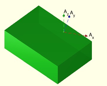
SGTget(SG,name)- returns a named frame of a solid geometry |
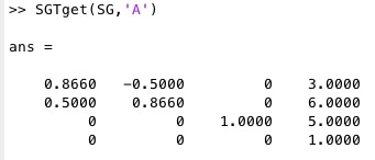 |
% SGTget(SG,name) - returns a named frame of a solid geometry % (by Tim Lueth, VLFL-Lib, 2016-JAN-05 as class: KINEMATICS AND FRAMES) % % returns the T transformation matrix for a named frame % (Status of: 2016-12-27) % % See also: SGTset, SGTplot, SGTremove, SGTui % % T=SGTget(SG,name) % === INPUT PARAMETERS === % SG: Solid Geometry % name: Name of required Frame % === OUTPUT RESULTS ====== % T: Frame matrix % % EXAMPLE: Return a previously set frame: % SG=SGbox([30,20,10]); SG=SGTset(SG,'A',TofDPhiH([3,6],pi/6,5)); % SGT(SG); % SGTget(SG,'A') % |
SGTset(SGN,N,T)- sets or replaces a named frame of a solid geometry |
 |
% SGTset(SGN,N,T) - sets or replaces a named frame of a solid geometry % (by Tim Lueth, VLFL-Lib, 2016-JAN-05 as class: KINEMATICS AND FRAMES) % % returns the updated SG including the new frame % (Status of: 2016-12-27) % % See also: SGTget, SGTplot, SGTremove, SGTui % % SGN=SGTset(SGN,N,T) % === INPUT PARAMETERS === % SGN: Solid Geometry % N: Name of required Frame % T: 4x4 matrix of the Frame % === OUTPUT RESULTS ====== % SGN: Frame matrix % % EXAMPLE: Set a HT Matrix % SG=SGbox([30,20,10]); SG=SGTset(SG,'A',TofDPhiH([3,6],pi/6,5)); SGT(SG) % |
patchupdateSG(h,SG,FL)- replaces an existing patch handle by updated SG |
 |
% patchupdateSG(h,SG,FL) - replaces an existing patch handle by updated SG % (by Tim Lueth, VLFL-Lib, 2016-JAN-04 as class: SURFACES) % % patchupdateSG(h,SG,[FL]) % === INPUT PARAMETERS === % h: existing patch handle % SG: Solid Geometry or VL % FL: optional Faces List % |
exp_2016_01_03a- EXPERIMENT to work in the direction of Chamfers |
 |
% exp_2016_01_03a - EXPERIMENT to work in the direction of Chamfers % % (by Tim Lueth, VLFL-Lib, 2016-JAN-03 as class: EXPERIMENTS) % % This experiment adds to all facets additional points near the vertices % and creates the missing facets. The absolute number of vertices ins % increased the number of facets is multiplied by 7! (Status of: % 2016-01-03) % % FL=exp_2016_01_03a % === OUTPUT RESULTS ====== % FL: % |
exp_2016_01_02a- EXPERIMENT to show the improvement of Radialedges |
 |
% exp_2016_01_02a - EXPERIMENT to show the improvement of Radialedges % (by Tim Lueth, VLFL-Lib, 2016-JAN-02 as class: EXPERIMENTS) % % exp_2016_01_02a % |
exp_2016_01_02- EXPERIMENT explaining appereance of noise |
 |
% exp_2016_01_02 - EXPERIMENT explaining appereance of noise % (by Tim Lueth, VLFL-Lib, 2016-JAN-02 as class: EXPERIMENTS) % % 'Details', 'Noise' arise from Boolean operations of polygons. % They have to be removed by % a) removing the details after the operation % b) understanding the rising of the problems (Status of: 2016-01-02) % % exp_2016_01_02 % |
exp_2016_01_01- EXPERIMENT to create a realtime system |
 |
% exp_2016_01_01 - EXPERIMENT to create a realtime system % (by Tim Lueth, RT-Lib, 2016-JAN-01 as class: EXPERIMENTS) % % Based on the procedures of 2011. After starting the procedure RTstart, % a Matlab shell with a new prompt will appear and allow the user to type % and use Matlab as before. Nevertheless some procedure are active in the % background. % 'STOP', 'QUIT', 'END', or "EXIT' will interrupt the execution (Status % of: 2016-01-01) % % exp_2016_01_01 % % EXAMPLE: Simply type: % exp_2016_01_01 % |
exp_2015_12_30- EXPERIMENT for a leightweight plate |
 |
% exp_2015_12_30 - EXPERIMENT for a leightweight plate % (by Tim Lueth, VLFL-Lib, 2015-DEZ-30 as class: EXPERIMENTS) % % exp_2015_12_30 % |
exp_2015_12_29a- EXPERIMENT that creates frame with radial edges |
 |
% exp_2015_12_29a - EXPERIMENT that creates frame with radial edges % (by Tim Lueth, VLFL-Lib, 2015-DEZ-29 as class: EXPERIMENTS) % % exp_2015_12_29a % |
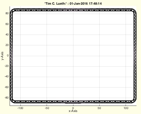
CPLfillHoneycomb(PLs,w,d,ww,n)- fills a contour with honeycomb |
 |
% CPLfillHoneycomb(PLs,w,d,ww,n) - fills a contour with honeycomb % (by Tim Lueth, VLFL-Lib, 2015-DEZ-29 as class: EXPERIMENTS) % % This procedure creates starting with [0 0] a honeycomb structure and % fills nested closed contours (Status of: 2015-12-29) % % CPL=CPLfillHoneycomb([PLs,w,d,ww,n]) % === INPUT PARAMETERS === % PLs: [x y] or closed contour of the border % w: width of the wall; default is 0.5 % d: distance between the walls % ww: width of the border wall; if ww<0 ; ww=distance to pattern % n: number of walls per cell; default is 6 % === OUTPUT RESULTS ====== % CPL: Closed contour that can be extruded by SGofCPLz % % EXAMPLE: Try: % CPLfillHoneycomb; % CPLfillHoneycomb(CPLsample(12)); % CPLfillHoneycomb(PLstar(40,12)); % CPLfillHoneycomb[100,30]); % |
exp_2015_12_29(PLs,w,d,ww,n)- EXPERIMENT to create lightweight boards |
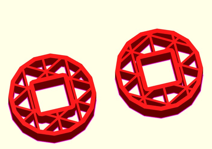 |
% exp_2015_12_29(PLs,w,d,ww,n) - EXPERIMENT to create lightweight boards % (by Tim Lueth, VLFL-Lib, 2015-DEZ-29 as class: EXPERIMENTS) % % Originally this procedure should create honey comp structures within a % square. Next step was to add the possibility to have an outer frame or % none. The last step was to allow different closed contours to create % honey comp structures inside. So the final example even works with % CPLsample(12). (Status of: 2015-12-29) % % CPL=exp_2015_12_29([PLs,w,d,ww,n]) % === INPUT PARAMETERS === % PLs: [x y] or closed contour of the border % w: width of the wall; default is 0.5 % d: distance between the walls % ww: width of the border wall; if ww<0 ; ww=distance to pattern % n: number of walls per cell; default is 6 % === OUTPUT RESULTS ====== % CPL: Closed contour that can be extruded by SGofCPLz % % EXAMPLE: Try: % exp_2015_12_29; % exp_2015_12_29(CPLsample(12)); % exp_2015_12_29(PLstar(40,12)); % exp_2015_12_29([100,30]); % |
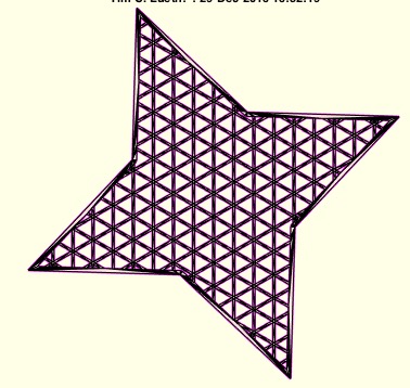
exp_2015_12_23- EXPERIMENT designing a bass cabinet for an IMPERIAL IIA accordion |
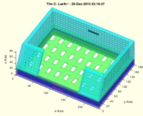 |
%% PUBLISHABLE EXP_2015_12_23 EXPERIMENT DESIGNING A BASS CABINET FOR AN IMPERIAL IIA ACCORDION % (by Tim Lueth, VLFL-Lib, 2015-DEZ-23 as class: EXPERIMENTS) %% % exp_2015_12_23 - EXPERIMENT designing a bass cabinet for an IMPERIAL % IIA accordion % (by Tim Lueth, VLFL-Lib, 2015-DEZ-23 as class: EXPERIMENTS) % % WORK in progess used to optimize the procedures CPL Pattern and % SGplatesofSGML. % The Frame 240*180 (Volume 80.65) had a weight of 98 gramm in Acryl -> % sw=1.22 % The Frame 120*180 (Volume 55.72) had a weight of 68 gramm in Acryl -> % sw=1.22 % The Frame 120*180 (Volume 55.72) had a weight of 51 gramm in PA -> % sw=0.92 % Since PA in in fact heavier than water (1.0), the density of PA is 80% % (Status of: 2015-12-26) % % exp_2015_12_23 % |
sbufferget(b,n)- reads bytes out of a struct buffer |
 |
% sbufferget(b,n) - reads bytes out of a struct buffer % (by Tim Lueth, VLFL-Lib, 2015-DEZ-08 as class: USB INTERFACE) % % the basic procedures are: % sbuffercreate - create a buffer % sbufferinfo - status info about the buffer % sbufferwrite - write data into the buffer % sbufferget - read data out of the buffer % (Status of: 2016-01-01) % % [b,rbytes,err]=sbufferget(b,n) % === INPUT PARAMETERS === % b: struct buffer % n: number of bytes to get % === OUTPUT RESULTS ====== % b: updated buffer % rbytes: array with received bytes % err: error number % |
sbufferwrite(b,mbytes)- writes bytes into a struct buffer |
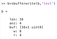 |
% sbufferwrite(b,mbytes) - writes bytes into a struct buffer % (by Tim Lueth, VLFL-Lib, 2015-DEZ-08 as class: USB INTERFACE) % % the basic fnctns are: % sbuffercreate - create a buffer % sbufferinfo - status info about the buffer % sbufferwrite - write data into the buffer % sbufferget - read data out of the buffer % (Status of: 2017-01-29) % % See also: sbuffercreate, sbufferinfo, sbufferget % % [b,err]=sbufferwrite(b,mbytes) % === INPUT PARAMETERS === % b: struct buffer % mbytes: bytes array to write % === OUTPUT RESULTS ====== % b: updated buffer % err: error number % |
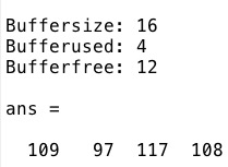
sbufferinfo(b)- returns information on a struct buffer |
 |
% sbufferinfo(b) - returns information on a struct buffer % (by Tim Lueth, VLFL-Lib, 2015-DEZ-08 as class: USB INTERFACE) % % the basic fnctns are: % sbuffercreate - create a buffer % sbufferinfo - status info about the buffer % sbufferwrite - write data into the buffer % sbufferget - read data out of the buffer % (Status of: 2017-01-29) % % See also: sbuffercreate, sbufferwrite, sbufferget % % [f,l,u]=sbufferinfo(b) % === INPUT PARAMETERS === % b: struct buffer % === OUTPUT RESULTS ====== % f: number of free bytes % l: maximum number of bytes % u: number of used bytes % |
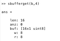
sbuffercreate(n)- creates a struct buffer for async read/write |
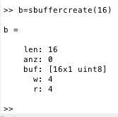 |
% sbuffercreate(n) - creates a struct buffer for async read/write % (by Tim Lueth, VLFL-Lib, 2015-DEZ-08 as class: USB INTERFACE) % % len = length of buffer % anz = number of used bytes of buffer % buf = data bytes of buffer % The basic procedures are: % sbuffercreate - create a buffer % sbufferinfo - status info about the buffer % sbufferwrite - write data into the buffer % sbufferget - read data out of the buffer % (Status of: 2016-01-01) % % b=sbuffercreate([n]) % === INPUT PARAMETERS === % n: number of bytes; default is 256 % === OUTPUT RESULTS ====== % b: buffer struct % |
exp_2015_12_08- Experiment that contains FIFO buffer handling |
 |
% exp_2015_12_08 - Experiment that contains FIFO buffer handling % (by Tim Lueth, VLFL-Lib, 2015-DEZ-08 as class: EXPERIMENTS) % % The procedures within this experiment are % sbuffercreate - create a buffer structure % sbufferinfo - return current buffer status % sbufferwrite - write data into the buffer % sbufferget - read data out of the buffer % (Status of: 2015-12-08) % % exp_2015_12_08 % |
exp_2015_12_07- writes an SG file with several planes for make things |
 |
% exp_2015_12_07 - writes an SG file with several planes for make things % (by Tim Lueth, VLFL-Lib, 2015-DEZ-07 as class: EXPERIMENTS) % % exp_2015_12_07 % |
CPLtextimage(text,dt,f,sx,sy,sz,ha)- returns contour of text string |
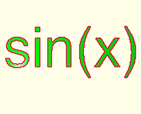 |
% CPLtextimage(text,dt,f,sx,sy,sz,ha) - returns contour of text string % (by Tim Lueth, VLFL-Lib, 2015-DEZ-07 as class: TEXT PROCEDURES) % % This is q quite generic but very slow procedure! (Status of: 2017-03-19) % % See also: CPLtextimage, VLFLtextimage, imageoftext, VLofimage, % textHorizontalBlockAlign, CPLoftext % % [CPL,VL,EL,FL]=CPLtextimage(text,[dt,f,sx,sy,sz,ha]) % === INPUT PARAMETERS === % text: Text String / Latex % dt: Pixel size; Default is 0.25 % f: Font size; Default is 72 % sx: Size in x; default is 0, i.e. no scaling % sy: Size in y; default is 0, i.e. no scaling % sz: Size in z; default is 0, i.e. no scaling % ha: horizontal alignment: 'l' or 'c' or 'r' % === OUTPUT RESULTS ====== % CPL: Closed Polygon List % VL: VertexLlist % EL: Edge List % FL: Facet List % % EXAMPLE: % CPLtextimage('sin(x)') % |
USBpololu- USB-communication with a Pololu Maestro Controller (Dual-Port Mode) |
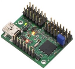 |
% USBpololu - USB-communication with a Pololu Maestro Controller (Dual-Port Mode) % (by Tim Lueth, VLFL-Lib, 2015-DEZ-01 as class: USB INTERFACE) % % To use the Pololu Maestro Boards with a MAC it is necessary to have % also a Windows/PC computer ready for downloading the 'Pololu Maestro % Control Center' that is available for Windows/PC only. You also need % the "Pololu Maestro Servo Controller User's Guide" as PDF-File % (https://www.pololu.com/docs/pdf/0J40/maestro.pdf). With respect to % page 47, the Maestro has to be set in **Dual-Port Mode**, which is very % easy using the Control Center but not possible without a Windows/PC. % The port with the smaller number is the command port on a Mac. % % The communication was tested successfully with ML2015b using Captain % OSX 10.11/MacBook Air 2011/MacBook Pro Retina Mid 2012 and a direct % connection to the Pololu Mini Maestro 12 Controller in sync mode using % fwrite and fread. It works also connected to a USB hub. % % You find distributors of Pololu at: https://www.pololu.com/distributors % Some distributors in Germany: % https://nodna.de, http://www.watterott.com, http://www.exp-tech.de % (Status of: 2015-12-02) % % See also: USBhelp, USBsearch % % USBpololu % |
USBsearch()- searches for specific USB serial devices on a MAC |
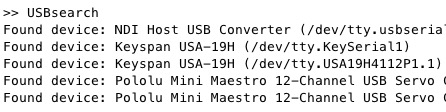 |
% USBsearch() - searches for specific USB serial devices on a MAC % (by Tim Lueth, VLFL-Lib, 2015-DEZ-01 as class: USB INTERFACE) % % On OSX/Mac all connected USB devices are detected by the command: % [~,out]=system('ioreg -p IOUSB') % Nevertheless, only if a device driver is installed, the device could be % found in the directory: % dir '/dev/tty*' % Therefor, this fnctn uses an array consisting of Device name, % Driver-Name, Driver source. % Afterwards, a serial port object is defined by % com1=serial('devicedriver') % Afterwards, this serial object is used to open or close a % fh=fopen(com1); fh=fclose(com1) % % Currently the following devices are supported: % - NDI Host USB Converter % - Pololu Mini Maestro 12-Channel USB Servo Controller % - Keyspan USA-19H % - Arduino Mega (Status of: 2017-01-29) % % See also: USBhelp, USBpololu % % USBsearch([]) % % EXAMPLE: just type % USBsearch: % Searches for a couple of useful USB serial devices % |
USBhelp- Help text for the use of USB serial communication on MAC |
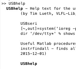 |
% USBhelp - Help text for the use of USB serial communication on MAC % (by Tim Lueth, VLFL-Lib, 2015-DEZ-01 as class: USB INTERFACE) % % Important OSX/Mac Darwin serial communication commands % [~,found]=system('ioreg -p IOUSB') % returns all USB devices attached % ls '/dev/tty*' % shows all existing devices with serial communication % % Useful Matlab fnctns: % instrfindall - finds all registered serial port objects (Status of: % 2017-01-29) % % Introduced first in SolidGeometry 2.8 % % See also: USBhelp, USBsearch, USBpololu % % USBhelp % % See also: USBhelp, USBsearch, USBpololu % |
exp_2015_12_01 (t)- EXPERIMENT for servo motor controller at OSX/Mac |
 |
% exp_2015_12_01 (t) - EXPERIMENT for servo motor controller at OSX/Mac % (by Tim Lueth, VLFL-Lib, 2015-DEZ-01 as class: USB INTERFACE) % % This file is also used as USBpololu_1 and USBpololu_2 % % To use the Pololu Maestro Boards with a MAC it is necessary to have % also a Windows/PC computer ready for downloading the 'Pololu Maestro % Control Center' that is available for Windows/PC only. You also need % the "Pololu Maestro Servo Controller User's Guide" as PDF-File % (https://www.pololu.com/docs/pdf/0J40/maestro.pdf). With respect to % page 47, the Maestro has to be set in **Dual-Port Mode**, which is very % easy using the Control Center but not possible without a Windows/PC. % With the Control Center, Timeout of the Pololu should be set to 0.00ms % (disable). You should also disable USB sleep mode. % On MAC, the port with the smaller number is the Command Port of the % Pololu. % % The communication was tested successfully with ML2015b using Captain % OSX 10.11/MacBook Air 2011/MacBook Pro Retina Mid 2012 and a direct % connection to the Pololu Mini Maestro 12 Controller in sync mode using % fwrite and fread. It works also connected to a USB hub. % % There is still a problem of Matlab using USB serial connections. After % 0.5-0.8 seconds, fwrite and fprint fails. % % You find distributors of Pololu at: https://www.pololu.com/distributors % Some distributors in Germany: % https://nodna.de, http://www.watterott.com, http://www.exp-tech.de % (Status of: 2015-12-04) % % exp_2015_12_01([t]) % === INPUT PARAMETERS === % t: target position % % EXAMPLE: exp_2015_12_01 (4000+1000*rand) % |
im2stereo (I1,I2)- returns corresponding points within 2 images taken from different view points |
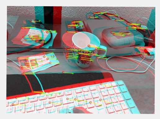 |
% im2stereo (I1,I2) - returns corresponding points within 2 images taken % from different view points % (by Tim Lueth, VLFL-Lib, 2015-NOV-25) % % This is just the implementation of the matlab example "Find % Corresponding Interest Points Between Pair of Images" that easy can be % used with an iPhone as ipcam. (Status of: 2015-11-25) % % im2stereo(I1,I2) % === INPUT PARAMETERS === % I1: RGB image 1 % I2: RGB image 1 % % EXAMPLE: fh=ipcam; I1=fh.CData; pause (2); % fh=ipcam; I2=fh.CData; % im2stereo(I1,I2) % |
- analyzes the current directory for the use of MATLAB Toolbox function |
 |
% - analyzes the current directory for the use of MATLAB Toolbox fnctn % (by Tim Lueth, VLFL-Lib, 2015-OKT-25 as class: AUXILIARY PROCEDURES) % % See also: depuseString, depuseTL, depuseToolbox, publishTL, pcodeTL, % depfunTL, pcodedirTL % % % % EXAMPLE: Check all VLFL_Examples for Toolbox use: % depuseToolbox ('VLFL_EX*.m') % |
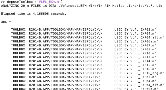
depuseToolbox(sstr)- analyzes the current directory for the use of MATLAB Toolbox procedure |
 |
% depuseToolbox(sstr) - analyzes the current directory for the use of MATLAB Toolbox procedure % (by Tim Lueth, VLFL-Lib, 2015-OKT-25 as class: AUXILIARY PROCEDURES) % % See also: depuseString, depuseTL, publishTL, pcodeTL, depfunTL, % pcodedirTL % % [TBFL,TL]=depuseToolbox([sstr]) % === INPUT PARAMETERS === % sstr: search string % === OUTPUT RESULTS ====== % TBFL: Toolbox procedure usage list % TL: Toolbox procedure list % % EXAMPLE: Check all VLFL_Examples for Toolbox use: % depuseToolbox ('VLFL_EX*.m') % |
exp_2015_10_16- EXAMPLE TO SHOW THE USE OF THE USB-VICRA-INTERFACE |
 |
%% PUBLISHABLE EXP_2015_10_16 EXAMPLE TO SHOW THE USE OF THE USB-VICRA-INTERFACE % (by Christian Dietz, VICRA, 2015-OKT-16 as class: EXPERIMENTS) %% % exp_2015_10_16 - EXAMPLE TO SHOW THE USE OF THE USB-VICRA-INTERFACE % (by Christian Dietz, VICRA, 2015-OKT-16 as class: EXPERIMENTS) % % exp_2015_10_16 % |
help ()- |
 |
% help () - % (by Christian Dietz, VICRA, 2015-OKT-20 as class: MECHANICAL PROCEDURES) % % Damit der RS232-USB-Wandler vom Betriebssystem erkannt wird, muss % folgender Treiber installiert werden. Eventuell ist ein Neustart nötig. % http://www.ftdichip.com/Drivers/VCP.htm (Status of: 2015-10-20) % % help() % |