New in SG-Lib 3.9
Last change of this page: 2017-07-24
SGTBB(SG)- replaces the complex surface geometry by a simplified bounding box |
 |
% SGTBB(SG) - replaces the complex surface geometry by a simplified bounding box % (by Tim Lueth, VLFL-Lib, 2017-JUN-29 as class: KINEMATICS AND FRAMES) % % Since SG can be very large structures, the call by value concept of % matlab is time consuming. This fnctn replaces the solid geometries by % its bounding box geometries relative to the base frame. % in Contrast to SGofBB or BBofSG this fnctn handles in addition the % frames that are required for cinematic chains (Status of: 2017-07-02) % % Introduced first in SolidGeometry 3.9 % % See also: SGTchain, SGTcalibchain, iscollofSG % % SGbb=SGTBB(SG) % === INPUT PARAMETERS === % SG: cell list of solid geometries % === OUTPUT RESULTS ====== % SGbb: cell list of bounding boxes % % See also: SGTchain, SGTcalibchain, iscollofSG % |
SGTframeChain(nums,extr,B,F)- returns a list of frame connections for a cell list if solids |
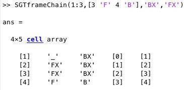 |
% SGTframeChain(nums,extr,B,F) - returns a list of frame connections for a cell list if solids % (by Tim Lueth, VLFL-Lib, 2017-JUN-26 as class: KINEMATICS AND FRAMES) % % Auxiliary fnctn called from SGTchain. The funxtion can be used to % create a frame-link-table of cell elements. The frame-link-table format % is % [BaseNr FFrame-SG1ind BFrame-SG2ind SG1ind SG2ind rot2nd ztr2nd] % BaseNr: Nr of SG in the final cell list; 0=origin % FFrame: Namestring of first (SG1ind) element's frame % BFrame: Namestring of second (SG2ind) element's frame % SG1ind: Index of first element in Geometry List SGc % SG2ind: Index of second element in Geometry List SGc % rot2nd: z-Rotation wrt to ez of BFrame of second element % ztr2nd: z-translation wrt to ez of BFrame of second element % (Status of: 2017-07-01) % % See also: SGTchain % % [LFrm,LL,Chstr]=SGTframeChain(nums,[extr,B,F]) % === INPUT PARAMETERS === % nums: number, or list of chain elements % extr: optional chaining; default is i-F -> i+1-B % B: extra chaining [SG1ind FFrame SG2ind BFrame] such as [1 'F' 2 'B'] % F: Standard Base frame string; default is 'B' % === OUTPUT RESULTS ====== % LFrm: Link Frame Tabe % LL: Link list [start index , End index] in SGc % Chstr: compiled string like the extra chaining % % EXAMPLE: % SGTframeChain(6) % SGTframeChain(1:3,'','BX','FX') % SGTframeChain(1:3,[3 'F' 4 'B'],'BX','FX') % SGTframeChain(1:7,[7 'F1' 8 'B' 7 'F2' 8 'B' 7 'F3' 8 'B']); % |
SGTsetorigin(SG,Nam)- moves the solid into a position that the base frame become the origin |
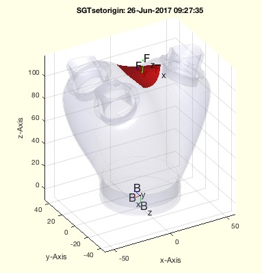 |
% SGTsetorigin(SG,Nam) - moves the solid into a position that the base frame become the origin % (by Tim Lueth, VLFL-Lib, 2017-JUN-26 as class: SURFACES) % % The position of the vertices and of the frames are moved (Status of: % 2017-06-26) % % See also: SGtransT, SGTget % % SGN=SGTsetorigin(SG,Nam) % === INPUT PARAMETERS === % SG: Solid geometry % Nam: Name of a frame % === OUTPUT RESULTS ====== % SGN: spatial transformed SG % % EXAMPLE: % load JACO_robot % SGTsetorigin(JCF,'B') % % |
SGpuzzlecut3D(SG,bsiz)- creates from a large solid geometry smaller printable parts |
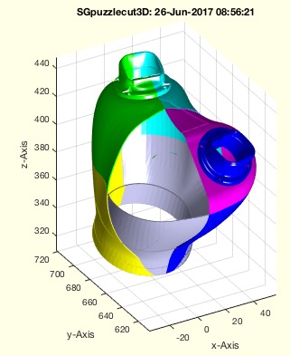 |
% SGpuzzlecut3D(SG,bsiz) - creates from a large solid geometry smaller printable parts % (by Tim Lueth, VLFL-Lib, 2017-JUN-25 as class: SURFACES) % % This fnctn helps to separate large Solids in smaller ones for printing % or for half-cuts of technical education (Status of: 2017-06-26) % % See also: SGsurfaceplot, SGwriteSeparatedSTL % % SGs=SGpuzzlecut3D(SG,[bsiz]) % === INPUT PARAMETERS === % SG: Solid Geometry % bsiz: [maxx maxy maxz]; if values are <=1 it is not the size but divider % === OUTPUT RESULTS ====== % SGs: List of puzzle elements % % EXAMPLE: % load JACO_robot.mat % SGpuzzlecut3D(JC6,[0.5 0.5 0.5]); % % h=patchofgca; setplotlight(h,'r',1) % |
isplanarVLFL(VL,FL,thre)- return whether a point cloud or surface is planar |
 |
% isplanarVLFL(VL,FL,thre) - return whether a point cloud or surface is planar % (by Tim Lueth, VLFL-Lib, 2017-JUN-25 as class: SURFACES) % % works with VL or VL/FL (Status of: 2017-06-25) % % Introduced first in SolidGeometry 3.9 % % See also: isconvexPL % % [r,m]=isplanarVLFL(VL,[FL,thre]) % === INPUT PARAMETERS === % VL: Vertex List % FL: optional Facet List to accelerate % thre: Optional threshold; default is 1e-2 ~ 1% % === OUTPUT RESULTS ====== % r: true if planar, i.e. m % % See also: isconvexPL % % % Copyright 2017 Tim C. Lueth |
VLFLsurfaceofSGT(SG,N,t,d,s)- returns the flange surface for a given T matrix frame name |
 |
% VLFLsurfaceofSGT(SG,N,t,d,s) - returns the flange surface for a given T matrix frame name % (by Tim Lueth, VLFL-Lib, 2017-JUN-25 as class: SURFACES) % % calls fnctn SGofSurface with the surfaces of Frame N (Status of: % 2017-06-25) % % Introduced first in SolidGeometry 3.9 % % See also: isplanarVLFL, SGofSurface % % [VL,FL]=VLFLsurfaceofSGT(SG,[N,t,d,s]) % === INPUT PARAMETERS === % SG: Solid Geometry % N: Name of Frame % t: thickness of the solid; default is 0.5 % d: distance from the surface; default is 0.3 % s: streching of the border line; default is 0 % === OUTPUT RESULTS ====== % VL: Vertex List % FL: Facet List % % EXAMPLE: % load JACO_robot.mat % X=SGTui(JC01,'T',1); % VLFLsurfaceofSGT(X,'T') % % See also: isplanarVLFL, SGofSurface % |
NLconformance(NVL,ez);- changes the orientation of a list of normal vectors |
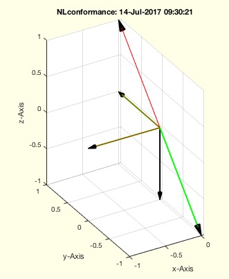 |
% NLconformance(NVL,ez); - changes the orientation of a list of normal vectors % (by Tim Lueth, VLFL-Lib, 2017-JUN-25 as class: ANALYTICAL GEOMETRY) % % in case that a vector has a relative angle of more than 90 degree % (pi/2) to ez, it is turned in direction (multiplied with -1) (Status % of: 2017-06-26) % % Introduced first in SolidGeometry 3.9 % % See also: NLcontourVL % % NVL=NLconformance(NVL,ez); % === INPUT PARAMETERS === % NVL: Normal vector list % ez: reference direction vector. % === OUTPUT RESULTS ====== % NVL: Correct normal vector list % % See also: NLcontourVL % |
cellstrfind(cellstr,str)- returns the position of a string in a cell list of string |
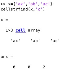 |
% cellstrfind(cellstr,str) - returns the position of a string in a cell list of string % (by Tim Lueth, VLFL-Lib, 2017-JUN-25 as class: AUXILIARY PROCEDURES) % % See also: cell2str, str2cell, cell2array % % f=cellstrfind(cellstr,str) % === INPUT PARAMETERS === % cellstr: cellstr % str: search string % === OUTPUT RESULTS ====== % f: array of position for each cell elememt % % EXAMPLE: % x={'ax','ab','ac'} % cellstrfind(x,'c') % |
CVLofRL(RL,ez)%- returns a CVL of a radial list and an ez vector |
 |
% CVLofRL(RL,ez)% - returns a CVL of a radial list and an ez vector % (by Tim Lueth, VLFL-Lib, 2017-JUN-22 as class: ANALYTICAL GEOMETRY) % % This fnctn can be used to postprocess an Radial list of % TR3mountingfaces or CVLdimclassifier % RL has the format: % [xc yc zc r n deg xs ys zs] % [xc yc zc] is the center of the circle % r is the radius % n is the number of found point % deg is the angle of the circle segment % [xs yz zs] can be either a sample point or the norm vector % (Status of: 2017-06-25) % % See also: CVLdimclassifier, TR3mountingfaces, SGTui % % CVL=CVLofRL(RL,[ez])% % === INPUT PARAMETERS === % RL: Radial list % ez: optional ez vector; or ez vector list list % === OUTPUT RESULTS ====== % CVL: Closed Vertex List % % EXAMPLE: % SG=SGtransR(SGsample(25),rot(pi/6,0,pi/2)); % TR3=triangulation(SG.FL,SG.VL); % [a,b,c,d,e]=TR3mountingfaces(TR3,23,1); show % CVL=CVLofRL(e,b); SGfigure; SGplot(SG); CVLplot(CVL); % |
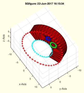
JACOstruct- creates a global struct JACOs that is used by JACOsim, JACOget, JACOset |
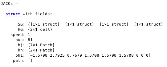 |
% JACOstruct - creates a global struct JACOs that is used by JACOsim, JACOget, JACOset % (by Tim Lueth, ROBOT-Lib, 2017-JUN-20) % % To use the global JACO struct, insert the following line into your % fnctn: % % global JACOs; JACOstruct; % Useage of global JACO robot struct % % It consist of: % JACOs.SG=SGreduceVLFL(JACO,3000); % Geometry of JACO % JACOs.HG={}; % Geometry of obstacles % JACOs.speed=1; % Robot speed % JACOs.bus=81; % Robot USB address % JACOs.hj=[]; % handle for drawing of robot % JACOs.hh=[]; % handle for environment drawing % JACOs.phi=[0 0 0 0 0 0 0 0 0]; % current Position % JACOs.path=[]; % current path % (Status of: 2017-06-21) % % See also: JACOget, JACOset, JACOsim % % JACOstruct % % EXAMPLE: inspect struct and current values % global JACOs; JACOstruct; % Useage of global JACO robot struct % JACOs % |
opponentFL(FL,fii)- returns the opponents indices for a facet list |
 |
% opponentFL(FL,fii) - returns the opponents indices for a facet list % (by Tim Lueth, VLFL-Lib, 2017-JUN-19 as class: SURFACES) % % NOT WELL TESTED YET! (Status of: 2017-06-19) % % OiL=opponentFL(FL,[fii]) % === INPUT PARAMETERS === % FL: Facet list % fii: optional index of facet % === OUTPUT RESULTS ====== % OiL: opponent of vertex i in facet fii % |
JACOset(CMD,PVAL)- sets parameter of the real JACO robot and of the global JACO model |
 |
% JACOset(CMD,PVAL) - sets parameter of the real JACO robot and of the global JACO model % (by Tim Lueth, ROBOT-Lib, 2017-JUN-19) % % ======================================================================= % WORK IN PROGRESS (2017-06-20) - NOT READY FOR FINAL RELEASE % ======================================================================= % % See also: JACOget, JACOsim % % [ANSW,t]=JACOset([CMD,PVAL]) % === INPUT PARAMETERS === % CMD: Command string % PVAL: Parameter Values als cell or numeric value % === OUTPUT RESULTS ====== % ANSW: % t: % |
JACOsim(CMD,PVAL)- Simulates the behaviour of the JACO robot |
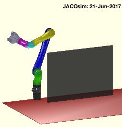 |
% JACOsim(CMD,PVAL) - Simulates the behaviour of the JACO robot % (by Tim Lueth, ROBOT-Lib, 2017-JUN-19) % % This fnctn is used to simulate the behavior of the JACO robot which is % helpful for visualization and collision detection and creating the % programatically interface of JACOget and JACOset and JACOstruc. % JACOsim supports the following commands: % 'init' = sets the JACOstruct to a predefined pose and 'shows' it % 'joints',phi = changes JACOStruct if the pose is collision free % 'show' = plots the pose of the joint values of JACOstruct % 'shows',phi = plots the pose of the given joint values % 'safe',{SG,'under'} = defines safety zones relative to JACO % 'stl', SGs = modifies the kinematic chain/geometry of the robot % JACOsim without an parameter => JACOsim('show') (Status of: 2017-06-21) % % See also: JACOget, JACOset, JACOstruct % % [ANSW,t]=JACOsim([CMD,PVAL]) % === INPUT PARAMETERS === % CMD: command string % PVAL: Parameter Values als cell or numeric value % === OUTPUT RESULTS ====== % ANSW: % t: % % EXAMPLE: % JACOsim('init') % Sets the simulation to a initial pose % JACOsim('safe',{A,'alignbottom','infront',-200,'left',0}) % safety zone % JACOsim,('stl',SG) % modifies the kinematic chain/geometry of the robot % |
nearestcluster(RL,lim)- returns a reduced list of points and a cluster list |
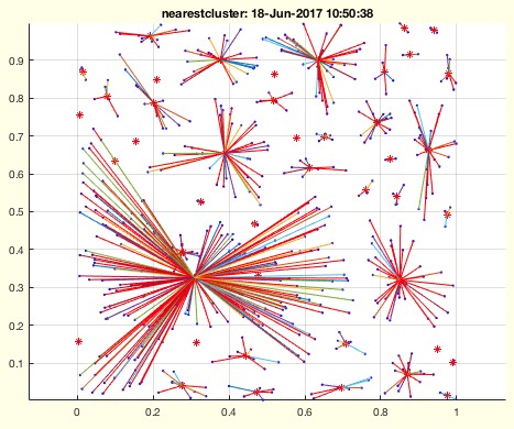 |
% nearestcluster(RL,lim) - returns a reduced list of points and a cluster list % (by Tim Lueth, VLFL-Lib, 2017-JUN-18 as class: ANALYTICAL GEOMETRY) % % Finds cluster of points with a minimal distance of lim; % draws a result only for [nx2 and nx3] % (Status of: 2017-06-18) % % See also: nearestpair, connectofmat % % [RLn,Rn]=nearestcluster(RL,lim) % === INPUT PARAMETERS === % RL: Point list % lim: maximum distance for clustering % === OUTPUT RESULTS ====== % RLn: Points list with replaced mean values % Rn: Cluster matrix related to RL % % EXAMPLE: % [a,b]=nearestcluster(rand(5,2),0.25) % nearestcluster(rand(500,2),0.05); % |
nofcolmap(col)- returns a number instead of a color string |
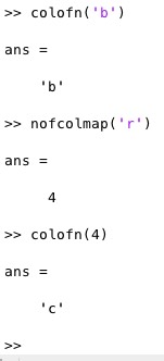 |
% nofcolmap(col) - returns a number instead of a color string % (by Tim Lueth, VLFL-Lib, 2017-JUN-17 as class: USER INTERFACE) % % colmap='kbgcrmyw'; % unfortunately, there is a fnctn color of matlab and tim lueth % (Status of: 2017-06-17) % % See also: colofn, color % % col=nofcolmap(col) % === INPUT PARAMETERS === % col: color integer od string % === OUTPUT RESULTS ====== % col: number of color % % EXAMPLE: % colofn('2') % nofcolmap('r') % |
SGreduceVLFL(SG,f)- returns a solid with reduced |
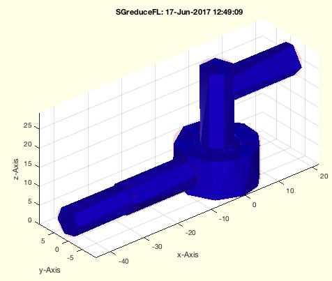 |
% SGreduceVLFL(SG,f) - returns a solid with reduced % (by Tim Lueth, VLFL-Lib, 2017-JUN-17 as class: SURFACES) % % speed optimized; uses reducepatch. % can be used to reduce facet related to the original vertex list (Status % of: 2017-06-17) % % See also: reducepatch, findVL % % [SG,FL,vi]=SGreduceVLFL(SG,[f]) % === INPUT PARAMETERS === % SG: Original Solid Geometry % f: reduction factor or number of facets per % === OUTPUT RESULTS ====== % SG: SG with reduced vertices and facets % FL: Facet List related to original solid geometry (slows down by findVL) % vi: index of new vertices related to original solid geometry % % EXAMPLE: % a=SGsample(17); a=SGstripfields(a) % SGreduceVLFL(a,800) % SGreduceVLFL(a,0.5) % [~,FL]=SGreduceVLFL(a,0.1), VLFLplot(a.VL,FL) % |
sofBB(SG,minv)- returns the maximal dimension of the bounding box |
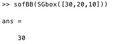 |
% sofBB(SG,minv) - returns the maximal dimension of the bounding box % (by Tim Lueth, VLFL-Lib, 2017-JUN-17 as class: AUXILIARY PROCEDURES) % % Useful fnctn for some SG plot fnctn (Status of: 2017-06-17) % % See also: sizeVL % % [ms,s]=sofBB(SG,[minv]) % === INPUT PARAMETERS === % SG: VL oder SG % minv: optional minimal value; default is 0 % === OUTPUT RESULTS ====== % ms: max dimension % s: [sx,sy,sz] % |
setplotlight(hi,col,alpha);- changes the alpha value of a given graphics object handle |
 |
% setplotlight(hi,col,alpha); - changes the alpha value of a given graphics object handle % (by Tim Lueth, VLFL-Lib, 2017-JUN-16 as class: VISUALIZATION) % % Similar to VLFLplotlight, but sets the parameter individually for a % patch handle (Status of: 2017-06-17) % % See also: VLFLplotlight % % setplotlight(hi,[col,alpha]); % === INPUT PARAMETERS === % hi: patch handle % col: color value or letter; optional % alpha: alpha index % % EXAMPLE: % SGfigure; [~,~,h]=SGsurfaceplot(SGsample(20)); view(-30,30); % setplotlight(h,'',0.4); show % setplotlight(h,'b',0.4); show % % % |
rcmod1(n,cx,sq)- return rows and colum for a given number and col length |
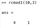 |
% rcmod1(n,cx,sq) - return rows and colum for a given number and col length % (by Tim Lueth, VLFL-Lib, 2017-JUN-16 as class: AUXILIARY PROCEDURES) % % Useful for subplot indi (Status of: 2017-06-16) % % See also: mod1, modn % % rc=rcmod1(n,cx,[sq]) % === INPUT PARAMETERS === % n: index % cx: number of cols % sq: if true; cx is the length of a squared field; default is false % === OUTPUT RESULTS ====== % rc: [row col] =[1... 1...] % |
SGTcalibchain(SGs,phi,Fram)- changes the base frames of a set of solid geoemtries |
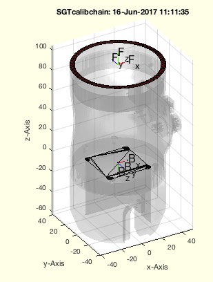 |
% SGTcalibchain(SGs,phi,Fram) - changes the base frames of a set of solid geoemtries % (by Tim Lueth, VLFL-Lib, 2017-JUN-16 as class: KINEMATICS AND FRAMES) % % This fnctn is useful if frames such as base frame or follower frame % were originally created manually from the STL files using SGTui but the % real frames have other orientations. % In this case, the fnctn SGTchain shows only the right pose for a set of % angles if an angle offset if added. If this offset angle is known, the % real configuration can be shown by SGTchain(offset) using the offset % angles. % To avoid the offset angle it is possible to calibrate the z axis of the % Base frame or the follower frame. (Status of: 2017-06-16) % % See also: SGTchain % % SGn=SGTcalibchain(SGs,[phi,Fram]) % === INPUT PARAMETERS === % SGs: Set of solids, with base and folloer frame % phi: offset angle for the % Fram: Frame name; default is 'B' % === OUTPUT RESULTS ====== % SGn: Set of solids, with turned frames % % EXAMPLE: % load JACO_robot.mat % SGTchain(JACO,[[0 0 -90 +180 +90 180 180]]/180*pi); view(-160,0); % % shows the zeros pose using an offset % X=SGTcalibchain(JACO,[[0 0 -90 +180 +90 180 180]]/180*pi) % turns the % base frames % SGTchain(X,[0 0 0 0 0 0 0]) % SGTchain(X,[0 0 180 180 0 0 0]/180*pi); view(-160,0) % |
iscollofSG(SGA,SGB,full,firstc,shape);- calculate collision vertices of two solids or a solid chain |
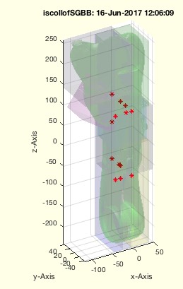 |
% iscollofSG(SGA,SGB,full,firstc,shape); - calculate collision vertices of two solids or a solid chain % (by Tim Lueth, VLFL-Lib, 2017-JUN-14 as class: KINEMATICS AND FRAMES) % % If result is empty; there is no collision % In case of (Status of: 2017-06-20) % % See also: SGreduceVLFL, VLcrossingSG % % res=iscollofSG(SGA,[SGB,full,firstc,shape]); % === INPUT PARAMETERS === % SGA: Solid A % SGB: Solid B; if empty SGA is used % full: true=full FL; false=Bounding box; default is false % firstc: true = stops after first crossings; false=complete; default=true % shape: if true; bounding boxe is relative to base frame; default=true % === OUTPUT RESULTS ====== % res: List of crossing points % |
isSG(SG)- return whether an object is a Solid Geometry |
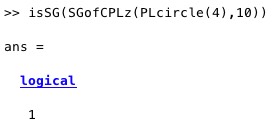 |
% isSG(SG) - return whether an object is a Solid Geometry % (by Tim Lueth, VLFL-Lib, 2017-JUN-14 as class: SURFACES) % % See also: isconvexPL, isPL % % res=isSG(SG) % === INPUT PARAMETERS === % SG: Object % === OUTPUT RESULTS ====== % res: result % % EXAMPLE: % isSG(PLcircle(4)) % isSG(SGofCPLz(PLcircle(4),2)) % |
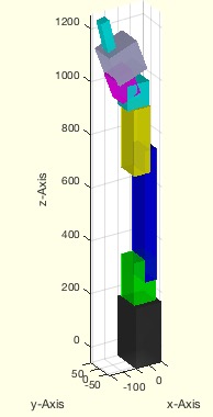
SGTchain(SGs,phi,z,nums,extr,B,F)- returns the spatial transformed solids of a kinematic chain |
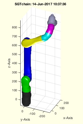 |
% SGTchain(SGs,phi,z,nums,extr,B,F) - returns the spatial transformed solids of a kinematic chain % (by Tim Lueth, VLFL-Lib, 2017-JUN-14 as class: KINEMATICS AND FRAMES) % % If no extra parameters are used, all connections are done using 'B' % Base frame and 'F' Follower Frame % The first rotation is currently ignored and can be called using NaN or % zeros. i.e. the base frame of the first element is always unchanged. % The parameter nums, extr, B and F are identical to SGTframechain to % define a the frame chain % for improved reaing and debugging it is possible to create a frame % chain once and use it as parameter nums (Status of: 2017-07-01) % % See also: SGTframeChain, SGTBB, SGTcalibchain, SGTplot, SGTui % % SGn=SGTchain(SGs,[phi,z,nums,extr,B,F]) % === INPUT PARAMETERS === % SGs: Cell list of n Solid Geometries % phi: vector of length n of radial rotations around the F-z frame % z: optional z value in ez direction % nums: optional chaining; nums can also be SGTframechain % extr: extra chaining [SG1ind FFrame SG2ind BFrame] such as [1 'F' 2 'B'] % B: Standard Base frame string; default is 'B' % F: Standard follower frame string; default is 'F' % === OUTPUT RESULTS ====== % SGn: Cell list of n spatial transformed Solid Geometries % % EXAMPLE: % load ('JACO_robot') % JACO={JC0,JC1,JC2,JC3,JC4,JC5,JC6} % SGfigure; SGplot(JACO); view(-30,30); show % SGTchain(JACO,[NaN pi/2]); % SGTchain(JACO,[NaN pi/1 pi/2 pi/3 pi/4 pi/5 pi/6]); % % a=JACOget('joints',1:6) % SGTchain(JACO,[+[NaN a]+[0 0 -90 +180 +90 180 180]]/180*pi); % view(-160,0) % ad=[-90 160 44 90 90 90]/180*pi; SGTchain(JACO,[NaN ad]); view(-160,0); % % Fchain=SGTframeChain(1:7,[7 'F' 8 'B' 7 'F2' 8 'B' 7 'F3' 8 'B']) % SGTchain(JACO,[NaN pi/2 pi pi],+100,Fchain) % % SGTchain([JACO,{JCF}],'','',false,1:7,[7 'F1' 8 'B' 7 'F2' 8 'B' 7 'F3' % 8 'B']) % |
JACOget(CMD,PVAL)- returns information on the JACO robot by direct calls |
 |
% JACOget(CMD,PVAL) - returns information on the JACO robot by direct calls % (by Tim Lueth & Samuel Detzel, ROBOT-Lib, 2017-JUN-13) % % ======================================================================= % WORK IN PROGRESS (2017-06-20) - NOT READY FOR FINAL RELEASE % ======================================================================= % % Commands are processed sequentially. % Therefor, if a specific jaco is called, use: % JACOget('jaco',2,'joints',1:6) to get the first six joints of jaco % Current commands are: % 'jaco' = number of jaco = [1...16] % 'joints' = get joint values = [1:9] (Status of: 2017-06-13) % % See also: PEAKinstall, JACOset, JACOsim % % [ANSW,t]=JACOget([CMD,PVAL]) % === INPUT PARAMETERS === % CMD: Command string % PVAL: Numeric Parameter Values % === OUTPUT RESULTS ====== % ANSW: Answer % t: time delay between call and answer % % EXAMPLE: Get information on the current joints of jaco #1 % JACOget('joints',1:3) % JACOget('jaco',2,'joints',1:9,'jaco',1,'joints',1:4) % |
SGof2CPLzbranch(CPLA,CPLB,z,stype,ctype)- Creates a Solid for an 1:n or n:1 solid branch |
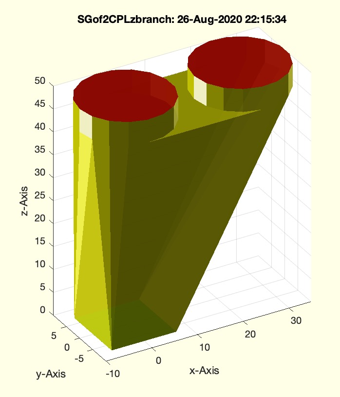 |
% SGof2CPLzbranch(CPLA,CPLB,z,stype,ctype) - Creates a Solid for an 1:n or n:1 solid branch % (by Tim Lueth, VLFL-Lib, 2017-JUN-12 as class: SURFACES) % % Creates a 1:n or n:1 solid branch. % Either CPLA or CPLB must consist of ONLY ONE contour (Status of: % 2017-06-13) % % See also: SGof2CPLz, SGof2CPLsz, SGof2CPLzheurist % % [SG,NFLW,NFLA,NFLB]=SGof2CPLzbranch([CPLA,CPLB,z,stype,ctype]) % === INPUT PARAMETERS === % CPLA: Contour A % CPLB: Contour B % z: height % stype: "number", "length", "angle", "center"; default is "length" % ctype: "mina" or "miny"; default is "mina" % % === OUTPUT RESULTS ====== % SG: Solid Geometry of the branch % NFLW: Wall Facets % NFLA: Bottom Facets % NFLB: Cover Facets % % EXAMPLE: % SGof2CPLzbranch(CPLsample(2), CPLsample(9),50) % SGof2CPLzbranch(CPLsample(6), CPLsample(10),50) % |
SGof2CPLzheurist(CPLA,CPLB,z,stype,ctype)- EXPERIMENT to show the connection of two contours |
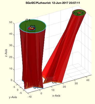 |
% SGof2CPLzheurist(CPLA,CPLB,z,stype,ctype) - EXPERIMENT to show the connection of two contours % (by Tim Lueth, VLFL-Lib, 2017-JUN-11 as class: SURFACES) % % This fnctn is the same as SGof2CPLsz but supports more than one % contour! The optimal result depends on the expectations of the user. % Consider different options for stype carefully: % "number" of points, i.e. 1:nmax % "length" of contour, i.e. 0:sum(edge length) % "angle" of contour, i.e. 0:sum(abs(edge angle)) % "center" of contour, i.e. 0:360 degree % also the starting point ctype ('rot' or 'min'); % Quite optimal procedure to find the walls between two planar contours % without adding new points. The number of faces is na+nb. % The resulting vertex list SG: % SG.VL=[VLaddz(CPA,0);VLaddz(CPB,z)]; % SG.FL=[FLA;FLB;FLW]; % (Status of: 2017-06-12) % % See also: SGof2CPLz, SGof2CPLsz, SGof2CPLzbranch, SGanalyzeGroupParts, % SGseparate, SGanalyzePenetration % % [SG,NFW,FLA,FLB,CC,LA,LB]=SGof2CPLzheurist([CPLA,CPLB,z,stype,ctype]) % === INPUT PARAMETERS === % CPLA: Contour A % CPLB: Contour B % z: height z % stype: "number", "length", "angle", "center"; default is "length" % ctype: "mina" or "miny"; default is "mina" % === OUTPUT RESULTS ====== % SG: New Vertex List % NFW: New Wall List % FLA: New Bottom FL % FLB: New TOP FL % CC: Correspondance list % LA: Index of Contours A in NVL % LB: Index of Contours B in NVL % % EXAMPLE: % SGof2CPLzheurist(CPLsample(14), CPLsample(26),'','angle'); % |
ELofCIL(CIL,cl)- Converts a Contour Index List into an Edge list |
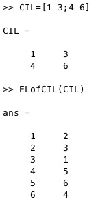 |
% ELofCIL(CIL,cl) - Converts a Contour Index List into an Edge list % (by Tim Lueth, VLFL-Lib, 2017-JUN-11 as class: AUXILIARY PROCEDURES) % % Contour index list [start index end index; start index end index ,...] % (Status of: 2017-06-11) % % See also: ELofn, CILofEL % % EL=ELofCIL(CIL,[cl]) % === INPUT PARAMETERS === % CIL: Contour index list [start index end index; start end ,...] % cl: closing; default is true % === OUTPUT RESULTS ====== % EL: Edge List % |
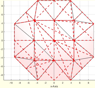
delaunayofCPL(CPLB)- more sharp delaunay triangulation |
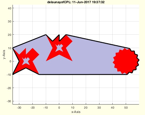 |
% delaunayofCPL(CPLB) - more sharp delaunay triangulation % (by Tim Lueth, VLFL-Lib, 2017-JUN-11 as class: CLOSED POLYGON LISTS) % % The delaunayTriangulation fnctn an be used to create a convex enclosing % facet. On the other hand, this convex contour also includes facets, % which are not necessary to enclose the original contours. % The fnctn also provides the edge list of the constricting contour. % (Status of: 2017-06-11) % % See also: delaunatTriangulation % % [TR3,oi,nfi,fi,EL]=delaunayofCPL(CPLB) % === INPUT PARAMETERS === % CPLB: Closed Contour List % === OUTPUT RESULTS ====== % TR3: delaunayTriangulation % oi: removed facets from outside % nfi: outside facets % fi: fi=isInterior(TR3) % % EL: Edge List of the % % EXAMPLE: % CPLB=[CPLsample(3)+[-25 0];NaN NaN;PLstar(10)+[0 10];NaN % NaN;PLstar(10)+[50 0]]; % |
VLofCVL(CVL)- creates a Contour index list for a CPL/CVL |
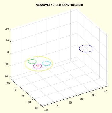 |
% VLofCVL(CVL) - creates a Contour index list for a CPL/CVL % (by Tim Lueth, VLFL-Lib, 2017-JUN-10 as class: CLOSED POLYGON LISTS) % % This is in fact the same fnctn as CILofCVL which is called in this % fnctn. % (Status of: 2017-06-10) % % Introduced first in SolidGeometry 3.9 % % See also: CVLofVLCIL % % [VL,CIL,EL]=VLofCVL(CVL) % === INPUT PARAMETERS === % CVL: CLosed Polygon list CPL/CVL % === OUTPUT RESULTS ====== % VL: Vertex list without doubles and NaNs % CIL: Contour index list related to VL % EL: % % EXAMPLE: % [VL,CIL]=VLofCVL(CPLsample(26)) % % See also: CVLofVLCIL % |
CILofCVL(CPL)- creates a Contour index list for a CPL/CVL |
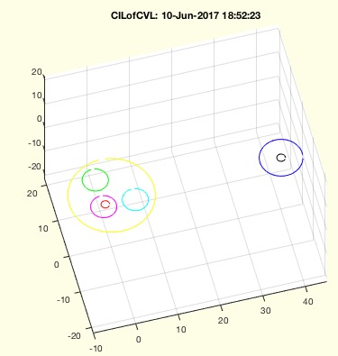 |
% CILofCVL(CPL) - creates a Contour index list for a CPL/CVL % (by Tim Lueth, VLFL-Lib, 2017-JUN-10 as class: CLOSED POLYGON LISTS) % % [CILC,VL,CIL]=CILofCVL(CPL) % === INPUT PARAMETERS === % CPL: CLosed Polygon list CPL/CVL % === OUTPUT RESULTS ====== % CILC: Contour index list related to CPL % VL: Vertex list without doubles and NaNs % CIL: Contour index list related to VL % % EXAMPLE: % [CILC,VL,CIL]=CILofCVL(CPLsample(26)) % |
cellofNaN(CVL)- converts a CVL/CPL into a cell list |
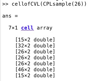 |
% cellofNaN(CVL) - converts a CVL/CPL into a cell list % (by Tim Lueth, VLFL-Lib, 2017-JUN-10 as class: AUXILIARY PROCEDURES) % % See also: selectNaN, separateNaN, replaceNaN % % VLcell=cellofNaN(CVL) % === INPUT PARAMETERS === % CVL: CVL/CPL separated by NaN % === OUTPUT RESULTS ====== % VLcell: Cell list of separated PL/CVL % % EXAMPLE: % cellofNaN(CPLsample(26)) % cellofNaN(CPLsample(27)) % |
CVLofVLCIL(VL,CIL)- returns a CPL/CVL from a PL or VL using a contour index list |
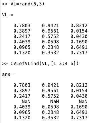 |
% CVLofVLCIL(VL,CIL) - returns a CPL/CVL from a PL or VL using a contour index list % (by Tim Lueth, VLFL-Lib, 2017-JUN-09 as class: CLOSED POLYGON LISTS) % % CIL= [startindex endindex; startindex endindex; ] % (Status of: 2017-06-09) % % See also: PLofCPL, CPLofPL, CILofCVL % % CVL=CVLofVLCIL(VL,CIL) % === INPUT PARAMETERS === % VL: Point or Vertex list % CIL: [startindex endindex; startindex endindex; ] % === OUTPUT RESULTS ====== % CVL: CLosed Polygon List or Closed Vertex List % % EXAMPLE: % VL=rand(6,3) % CVLofVLCIL(VL,[1 3;4 6]) % |
reversesortindex(iO)- returns the reverse sort index for a sort index |
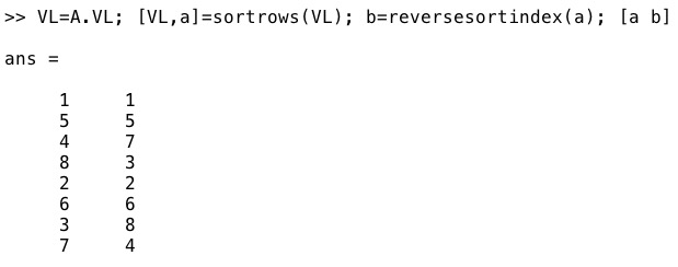 |
% reversesortindex(iO) - returns the reverse sort index for a sort index % (by Tim Lueth, VLFL-Lib, 2017-JUN-09 as class: AUXILIARY PROCEDURES) % % rO=sortrows([iO [1:size(iO)]']); rO=rO(:,2); (Status of: 2017-06-09) % % See also: maprows, findVL % % rO=reversesortindex(iO) % === INPUT PARAMETERS === % iO: result of sortrows % === OUTPUT RESULTS ====== % rO: reverse sort order % % EXAMPLE: % A=SGbox([30 20 10]); % VL=A.VL, [VL,a]=sortrows(VL), b=reversesortindex(a) % SGfigure; VLFLplot(VL,b(FL),'y'); % |
exp_2017_06_07(CPLA,CPLB,z)- EXPERIMENT to show the connection of two contours => SGof2CPLzheurist |
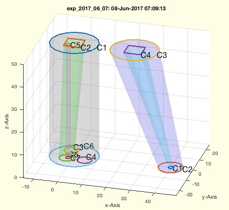 |
% exp_2017_06_07(CPLA,CPLB,z) - EXPERIMENT to show the connection of two contours => SGof2CPLzheurist % (by Tim Lueth, VLFL-Lib, 2017-JUN-08 as class: EXPERIMENTS) % % This fnctn is the same as SGof2CPLz but supports more than one contour! % The optimal result depends on the expectations of the user. Consider % different options for stype carefully: % "number" of points, i.e. 1:nmax % "length" of contour, i.e. 0:sum(edge length) % "angle" of contour, i.e. 0:sum(abs(edge angle)) % "center" of contour, i.e. 0:360 degree % also the starting point ctype ('rot' or 'min'); % Quite optimal procedure to find the walls between two planar contours % without adding new points. The number of faces is na+nb. % The resulting vertex list SG: % SG.VL=[VLaddz(CPA,0);VLaddz(CPB,z)]; % SG.FL=[FLA;FLB;FLW]; % (Status of: 2017-06-12) % % [NVL,NFW,FLA,FLB,CC,LA,LB]=exp_2017_06_07([CPLA,CPLB,z]) % === INPUT PARAMETERS === % CPLA: Contour A % CPLB: Contour B % z: height z % === OUTPUT RESULTS ====== % NVL: New Vertex List % NFW: New Wall List % FLA: New Bottom FL % FLB: New TOP FL % CC: Correspondance list % LA: Index of Contours A in NVL % LB: Index of Contours B in NVL % % EXAMPLE: % [VL,FL,FLB,FLB,CC,LA,LB]=exp_2017_06_07(CPLsample(12),CPLsample(13)) % |
maxmax(A)- returns the maximal maximum of a multidimensional matrix |
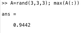 |
% maxmax(A) - returns the maximal maximum of a multidimensional matrix % (by Tim Lueth, VLFL-Lib, 2017-JUN-05 as class: AUXILIARY PROCEDURES) % % ======================================================================= % OBSOLETE (2017-06-05) - USE FAMILY 'max(D(:))' INSTEAD % ======================================================================= % % See also: [ max(D(:)) ] ; maxmax, minmin % % M=maxmax(A) % === INPUT PARAMETERS === % A: matrix % === OUTPUT RESULTS ====== % M: largest maximum of A % % EXAMPLE: % maxmax(rand(2,2,2)) % |
minmin(A)- returns the minimal minum of a multidimensional matrix |
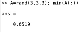 |
% minmin(A) - returns the minimal minum of a multidimensional matrix % (by Tim Lueth, VLFL-Lib, 2017-JUN-05 as class: AUXILIARY PROCEDURES) % % ======================================================================= % OBSOLETE (2017-06-05) - USE FAMILY 'min(D(:))' INSTEAD % ======================================================================= % % See also: [ min(D(:)) ] ; maxmax % % M=minmin(A) % === INPUT PARAMETERS === % A: matrix % === OUTPUT RESULTS ====== % M: min(min(..... % % EXAMPLE: % minmin(rand(2,2,2)) % |
removeimat(D,r,c)- removes a row and a column of a indexed matrix |
 |
% removeimat(D,r,c) - removes a row and a column of a indexed matrix % (by Tim Lueth, VLFL-Lib, 2017-JUN-05 as class: AUXILIARY PROCEDURES) % % See also: imat % % ND=removeimat(D,r,c) % === INPUT PARAMETERS === % D: indexed matrix % r: row to delete % c: column to delete % === OUTPUT RESULTS ====== % ND: Matrix without this column and row % % EXAMPLE: % D=imat(rand(3,5)), removeimat(D,1,2) % |
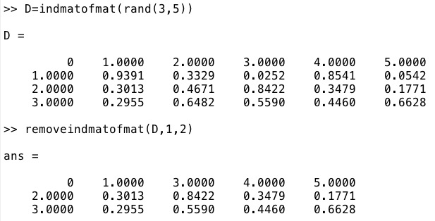
imat(D)- returns a matrix including row column and column row |
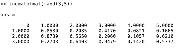 |
% imat(D) - returns a matrix including row column and column row % (by Tim Lueth, VLFL-Lib, 2017-JUN-05 as class: AUXILIARY PROCEDURES) % % See also: imat, removeimat % % DN=imat(D) % === INPUT PARAMETERS === % D: matrix 2x2 % === OUTPUT RESULTS ====== % DN: matrix plus row column and column row % % EXAMPLE: % D=imat(rand(3,5)) % |
textCVL (CVL,c,s,nt,lb)- plots descriptors for each contour into a figure using text command |
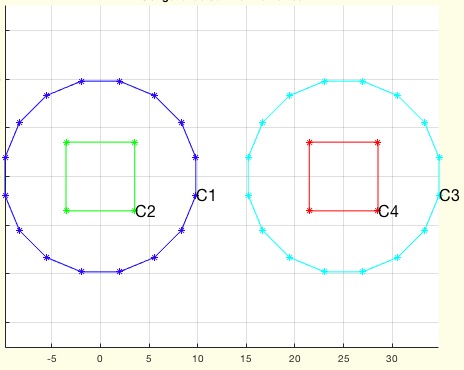 |
% textCVL (CVL,c,s,nt,lb) - plots descriptors for each contour into a figure using text command % (by Tim Lueth, VLFL-Lib, 2017-JUN-05 as class: VISUALIZATION) % % up to 99 contours are marked at the first point by a letter and a % number (Status of: 2017-06-05) % % See also: textT, textP, textVL % % textCVL(CVL,[c,s,nt,lb]) % === INPUT PARAMETERS === % CVL: Contour list separated by Nan (CPL/CVL) % c: Color, default is black % s: Size, default is 16 % nt: optional list of selected contours % lb: optional string for text; default is 'C' % % EXAMPLE: Different examples for plotting % SGfigure; CPL=CPLsample(12); CVLplot(CPL); textCVL(CPL); % |
nearestpair(PLA,PLB,tp);- returns the nearest point pairs of two vector list |
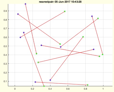 |
% nearestpair(PLA,PLB,tp); - returns the nearest point pairs of two vector list % (by Tim Lueth, VLFL-Lib, 2017-JUN-04 as class: ANALYTICAL GEOMETRY) % % Two vector list are processed using the norm distance. If the parameter % 'unique' is used, then e vector that was used already cannot be used a % second time. The index zero shows that there is no corresponding vector % in the second list (Status of: 2017-06-18) % % See also: nearestcluster, connectofmat, norm, PLcorrelate, CPLcorrelate % % [p,x,D]=nearestpair(PLA,PLB,[tp]); % === INPUT PARAMETERS === % PLA: Vector list A % PLB: Vector list B % tp: 'min', 'mean' ; default is 'min' % === OUTPUT RESULTS ====== % p: index in B for each point of A % x: Distance between the pairs % D: Full Distance matrix % % EXAMPLE: % D1=rand(10,2); D2=rand(10,2); % nearestpair(D1,D2,'mean'); % nearestpair(D1,D2,'min'); % |
circshiftCPL(CPL,n)- returns a circular shifted CPL |
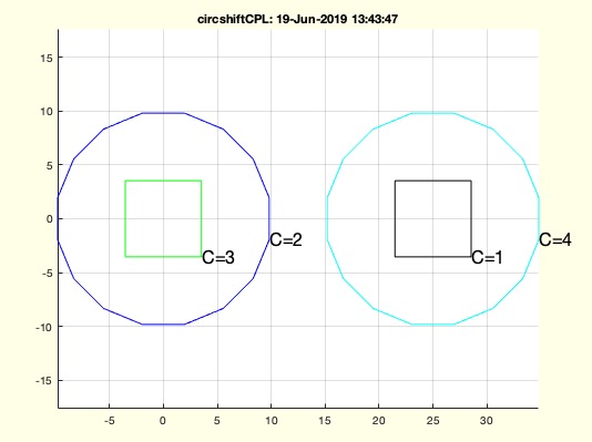 |
% circshiftCPL(CPL,n) - returns a circular shifted CPL % (by Tim Lueth, VLFL-Lib, 2017-JUN-04 as class: CLOSED POLYGON LISTS) % % This is more or less for testing CPLcorrelate (Status of: 2017-06-04) % % See also: CPLcircshift % % CPL=circshiftCPL(CPL,[n]) % === INPUT PARAMETERS === % CPL: Closed Polygon List % n: number of circshifts polygon; default is random % === OUTPUT RESULTS ====== % CPL: resulting CPL % % EXAMPLE: % SGfigure; B=circshiftCPL(CPLsample(13)) ;CVLplot(circshiftCPL(B)); % SGfigure; B=circshiftCPL(CPLsample(14)) ;CVLplot(circshiftCPL(B)); % |
CPLcorrelate(CPLA,CPLB)- correlates the contours from two CPLs |
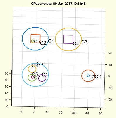 |
% CPLcorrelate(CPLA,CPLB) - correlates the contours from two CPLs % (by Tim Lueth, VLFL-Lib, 2017-JUN-04 as class: CLOSED POLYGON LISTS) % % In contrast to PLcorrelate, which correlates points for a single pair % of a single contour, this fnctn here correlates contours to preprare % the use of PLcorrelate. The correlation List containts in each row the % corresponding contours of A and B, the level of the contour (0=most % outside) and the parent contour of Ai and the parent contour of Bi % The parameter list constains: % the row number, the parent, the level and the center point (Status of: % 2017-06-07) % % See also: FLofPLcorrelation, PLcorrelate, textCVL % % [CLL,a,b]=CPLcorrelate(CPLA,CPLB) % === INPUT PARAMETERS === % CPLA: Contour A % CPLB: Contour B % === OUTPUT RESULTS ====== % CLL: Correlation list [ACi BCi Level PAi PBi] % a: complete list of used parameter of a % b: complete list of used parameter of a % % EXAMPLE: % CPLcorrelate(CPLsample(26),CPLsample(27)) % CPLcorrelate(CPLsample(27),CPLsample(26)) % |
modN(n,k,N)- returns mod function for elements N:N+k(-1) |
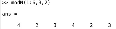 |
% modN(n,k,N) - returns mod fnctn for elements N:N+k(-1) % (by Tim Lueth, VLFL-Lib, 2017-JUN-04 as class: AUXILIARY PROCEDURES) % % auxiliary fnctn for array manipulation. Instead of return values % between [0..k-1], this fnctn returns [N..N+k-1] by a=mod(n-N,k)+N % (Status of: 2017-06-04) % % See also: mod1, mod % % a=modN(n,k,[N]) % === INPUT PARAMETERS === % n: number % k: divider % N: Interval start % === OUTPUT RESULTS ====== % a: rest % % EXAMPLE: % modN(1:6,3) % modN(1:6,3,2) % |
FLofPLcorrelation(CL,offset,VL)- returns a facet list for a given point correspondance list |
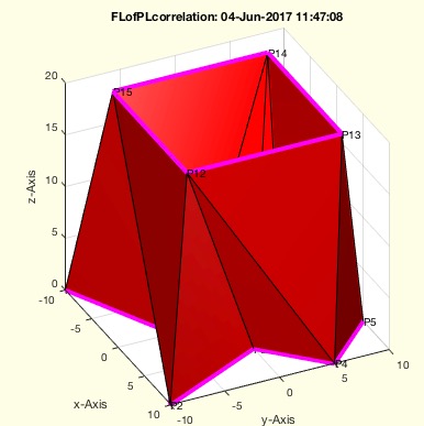 |
% FLofPLcorrelation(CL,offset,VL) - returns a facet list for a given point correspondance list % (by Tim Lueth, VLFL-Lib, 2017-JUN-02 as class: SURFACES) % % See also: PLcorrelate % % FL=FLofPLcorrelation(CL,[offset,VL]) % === INPUT PARAMETERS === % CL: Correspondance list % offset: % VL: optional vertex list for a drawing % === OUTPUT RESULTS ====== % FL: Facet list created by the correspondance list % % EXAMPLE: % [CL,VL]=PLcorrelate(CPLsample(3),PLcircle(10,4)); % FLofPLcorrelation(CL,'',VL); % |
CPLconvexseg(CPL)- returns the segments of convex and concave contours a CPL. |
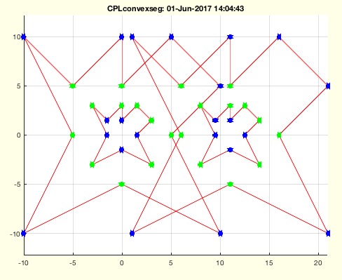 |
% CPLconvexseg(CPL) - returns the segments of convex and concave contours a CPL. % (by Tim Lueth, VLFL-Lib, 2017-JUN-01 as class: ANALYTICAL GEOMETRY) % % ATTENTION. Convex and concave are related to ccw orientation % +1 = convex (for ccw) [= concave for cw] % -1 = concave (for ccw) [= convex for cw] % Same fnctn as PLconvexseg for NAN separated CPLs (Status of: 2017-06-01) % % See also: isconvexPL, PLconvexseg % % con=CPLconvexseg(CPL) % === INPUT PARAMETERS === % CPL: Single Point List % === OUTPUT RESULTS ====== % con: array of convex and concave % % EXAMPLE: % CPLconvexseg(PLcircle(10,6)) % CPLconvexseg(flipud(PLcircle(10,6))) % PLconvexseg(PLsample(9)) % |
PLconvexseg(PL)- returns the segments of convex and concave conoturs within ONE CPL |
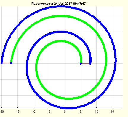 |
% PLconvexseg(PL) - returns the segments of convex and concave conoturs within ONE CPL % (by Tim Lueth, VLFL-Lib, 2017-JUN-01 as class: ANALYTICAL GEOMETRY) % % ATTENTION. Convex and concave are related to ccw orientation % +1 = convex (for ccw) [= concave for cw] % -1 = concave (for ccw) [= convex for cw] % Same fnctn as CPLconvexseg for single PL (Status of: 2017-07-24) % % Introduced first in SolidGeometry 3.9 % % See also: isconvexPL, CPLconvexseg, CPLisccwcorrected % % [con,AL,CIL]=PLconvexseg(PL) % === INPUT PARAMETERS === % PL: Single Point List % === OUTPUT RESULTS ====== % con: array of convex and concave % AL: Angle List % CIL: Change index list plus status [n x 3] % % EXAMPLE: % PLconvexseg(CPLsample(3)); % PLconvexseg(PLsample(9)); % PLconvexseg(CPLisccwcorrected(PLsample(9))); % % See also: isconvexPL, CPLconvexseg, CPLisccwcorrected % % % Copyright 2017 Tim C. Lueth |
replacemat(A,valold,valnew)- replaces values in vectors and matrices |
 |
% replacemat(A,valold,valnew) - replaces values in vectors and matrices % (by Tim Lueth, VLFL-Lib, 2017-JUN-01 as class: AUXILIARY PROCEDURES) % % mainly: A(A==valold(i))=valnew(i) % tab(mat) (Status of: 2017-06-01) % % replacemat(A,valold,valnew) % === INPUT PARAMETERS === % A: vectors or matrices % valold: existing values % valnew: new values % % EXAMPLE: % A=[1 2 3; 4 5 6], replacemat(A,1,9) % A=[1 2 3; 4 5 6], replacemat(A,[1 9],[9 0]) % |
distofintervall(a,b,inter)- distance within an intervall |
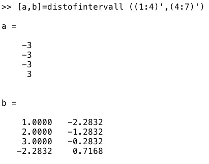 |
% distofintervall(a,b,inter) - distance within an intervall % (by Tim Lueth, VLFL-Lib, 2017-MAI-31 as class: AUXILIARY PROCEDURES) % % maps a value in circular intervall (Status of: 2017-05-31) % % See also: norm % % [d,iv]=distofintervall(a,b,[inter]) % === INPUT PARAMETERS === % a: value 1 % b: value 2 % inter: intervall; default is [-pi +pi] % === OUTPUT RESULTS ====== % d: distance () % iv: value a in intervall % % EXAMPLE: % a=distofintervall (-pi+pi/10,pi-pi/10) % a=distofintervall (1:10,2:11) % |
PLminangle(PL,in0,C,at)- returns the point with minimal angle value wrt to the center of the contour |
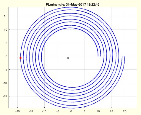 |
% PLminangle(PL,in0,C,at) - returns the point with minimal angle value wrt to the center of the contour % (by Tim Lueth, VLFL-Lib, 2017-MAI-31 as class: AUXILIARY PROCEDURES) % % See also: PLminyx % % [P,pin,AL,DL,C]=PLminangle(PL,[in0,C,at]) % === INPUT PARAMETERS === % PL: Point Liste % in0: false=[-pi..+pi]; true=[0..2*pi]; default is false % C: optional center point % at: angle threshold; default is pi/100 % === OUTPUT RESULTS ====== % P: Point with minimal y and minimal x % pin: find index in PL % AL: Angle list % DL: Distance from Center List % C: Center Point % % EXAMPLE: % PLminangle(CPLspiral(10,20,8*pi)) % PLminabgle(CPLspiral(10,20,8*pi),true) % PLminangle(CPLspiral(10,20,8*pi),true,[0 0]) % [~,ci]=PLminyx(CPLB); CPLB=circshift(CPLB,-(ci-1)); % |
PLcorrelate(PLA,PLB,stype,ctype,mtype)- returns the correlation of two single point lists |
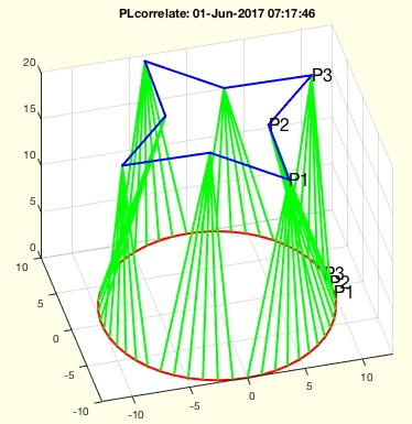 |
% PLcorrelate(PLA,PLB,stype,ctype,mtype) - returns the correlation of two single point lists % (by Tim Lueth, VLFL-Lib, 2017-MAI-31 as class: CLOSED POLYGON LISTS) % % Auxiliary fnctn to correlate two point lists. It was designed first in % SGof2CPLz. % SGof2CPLz is still more powerful. (Status of: 2017-06-04) % % See also: SGof2CPLz, FLofPLcorrelation, CPLcorrelate % % [CL,VL]=PLcorrelate([PLA,PLB,stype,ctype,mtype]) % === INPUT PARAMETERS === % PLA: Point list A % PLB: Point list B % stype: 'number','length','angle','center','nearest', default 'center' % ctype: 'org','minx','mina'/'rot'; default is 'mina' % mtype: 'none', 'norm', 'norm1' % === OUTPUT RESULTS ====== % CL: Correlation List % VL: Vertex list [PLA;PLAB] without doubled points % % EXAMPLE: % PLcorrelate(CPLsample(3),circshift(PLofCPL(CPLsample(3)),1)) % PLcorrelate(PLcircle(15),CPLsample(3)) % |
SGofCPLzchamfer(CPL,z,ph,ed);- returns a solid with chamfered edges |
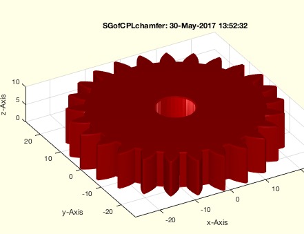 |
% SGofCPLzchamfer(CPL,z,ph,ed); - returns a solid with chamfered edges % (by Tim Lueth, VLFL-Lib, 2017-MAI-30 as class: SURFACES) % % Based on a comment of Florian Schleich. The body is divided into three % planes. In order to ensure the calculation of the walls, the % orientations of the contour are first adapted. (Status of: 2017-05-30) % % See also: SGofCPLz, SGof2CPLsz % % SG=SGofCPLzchamfer([CPL,z,ph,ed]); % === INPUT PARAMETERS === % CPL: Closed Polygon line % z: Height z % ph: phase default is 0.3 % ed: curved edges; default is true % === OUTPUT RESULTS ====== % SG: Resulting solid % % EXAMPLE: % SGofCPLchamfer([CPLsample(21);NaN NaN;PLcircle(5)],10) % SGofCPLzchamfer % % |
CPLisccwcorrected(CPL)- returns a CPL with all CPLs in correct orientation cw/ccw |
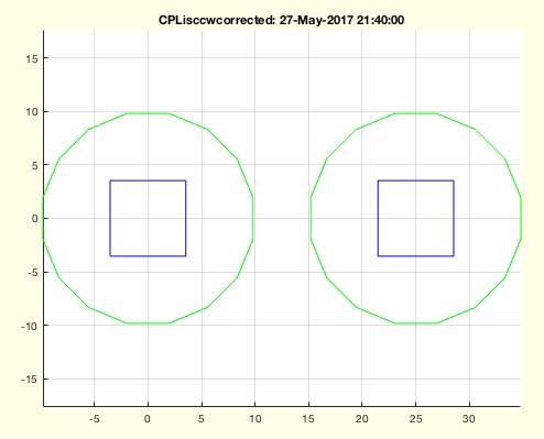 |
% CPLisccwcorrected(CPL) - returns a CPL with all CPLs in correct orientation cw/ccw % (by Tim Lueth, VLFL-Lib, 2017-MAI-27 as class: CLOSED POLYGON LISTS) % % See also: CPLisccw, CPLsortinout, CPLisccwinout % % [CPL,cio]=CPLisccwcorrected([CPL]) % === INPUT PARAMETERS === % CPL: Original CPL % === OUTPUT RESULTS ====== % CPL: Corrected CPL % cio: inside outside index % |
CPLisccwinout(CPL)- returns which contour has the right orientation wrt shell and orientation |
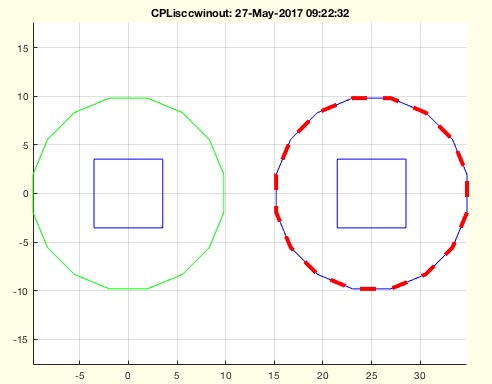 |
% CPLisccwinout(CPL) - returns which contour has the right orientation wrt shell and orientation % (by Tim Lueth, VLFL-Lib, 2017-MAI-27 as class: CLOSED POLYGON LISTS) % % Depending on the outwards level, the orientation of a contour is: % 0 = outward = ccw % 1 = inward = cw % 2 = outward = ccw % 3 ..... % if length(corr)==sum(corr); the contour is correct (Status of: % 2017-05-27) % % See also: CPLisccw, CPLsortinout, CPLisccwcorrected % % [corr,cio,ccw]=CPLisccwinout(CPL) % === INPUT PARAMETERS === % CPL: Contour polygon list % === OUTPUT RESULTS ====== % corr: true if correct % cio: level of contour (0=most outwards) % ccw: ccw direction % % EXAMPLE: % FCPL=replaceNaN(CPLsample(12),3,flipud(separateNaN(CPLsample(12),3))); % CPLisccwinout(FCPL) % CPLisccwinout(CPLsample(13)) % |
replaceNaN(CPL,ci,CPLi)- replaces a contour within a CPL |
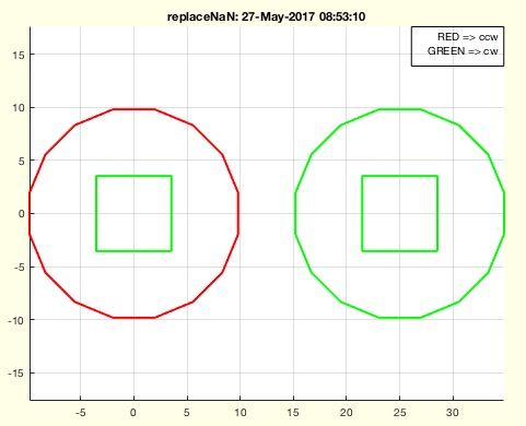 |
% replaceNaN(CPL,ci,CPLi) - replaces a contour within a CPL % (by Tim Lueth, VLFL-Lib, 2017-MAI-27 as class: CLOSED POLYGON LISTS) % % Introduced first in SolidGeometry 3.9 % % See also: selectNaN, separateNaN, cellofNaN % % CPL=replaceNaN(CPL,ci,CPLi) % === INPUT PARAMETERS === % CPL: CPL % ci: index of contour % CPLi: new contour for contour ci % === OUTPUT RESULTS ====== % CPL: % % EXAMPLE: % replaceNaN(CPLsample(12),3,flipud(separateNaN(CPLsample(12),3))); % % See also: selectNaN, separateNaN, cellofNaN % |
CVLseparatez(CVL,z,thr)- returns a sliced CVL/CPL for a given z value |
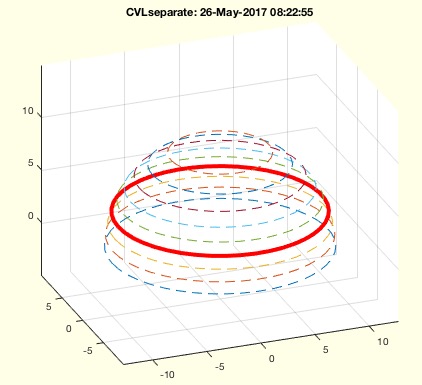 |
% CVLseparatez(CVL,z,thr) - returns a sliced CVL/CPL for a given z value % (by Tim Lueth, VLFL-Lib, 2017-MAI-26 as class: CLOSED POLYGON LISTS) % % for sliced CVL, i.e. CPL with an added z value, this fnctn returns only % the contours that have the same z value (Status of: 2017-07-23) % % Introduced first in SolidGeometry 3.9 % % See also: CVLofSGslices, SGofCVLslices % % [CVLz,zL]=CVLseparatez(CVL,[z,thr]) % === INPUT PARAMETERS === % CVL: Slices CVL % z: desired z value; currently only scalar % thr: tolerance for finding a z value % === OUTPUT RESULTS ====== % CVLz: Contours that fulfill the z-value condition; separated by NaN OR % zl if isempty(z) % zL: List of z Values % % EXAMPLE: % CVL=CVLofSGslices(SGsample(5),10); % CVLseparatez(CVL,3.3333333); % % See also: CVLofSGslices, SGofCVLslices % % % Copyright 2017 Tim C. Lueth |